Wildfires in the West

The second largest fire in Colorado's History is currently burning. California is also having a historic fire season.

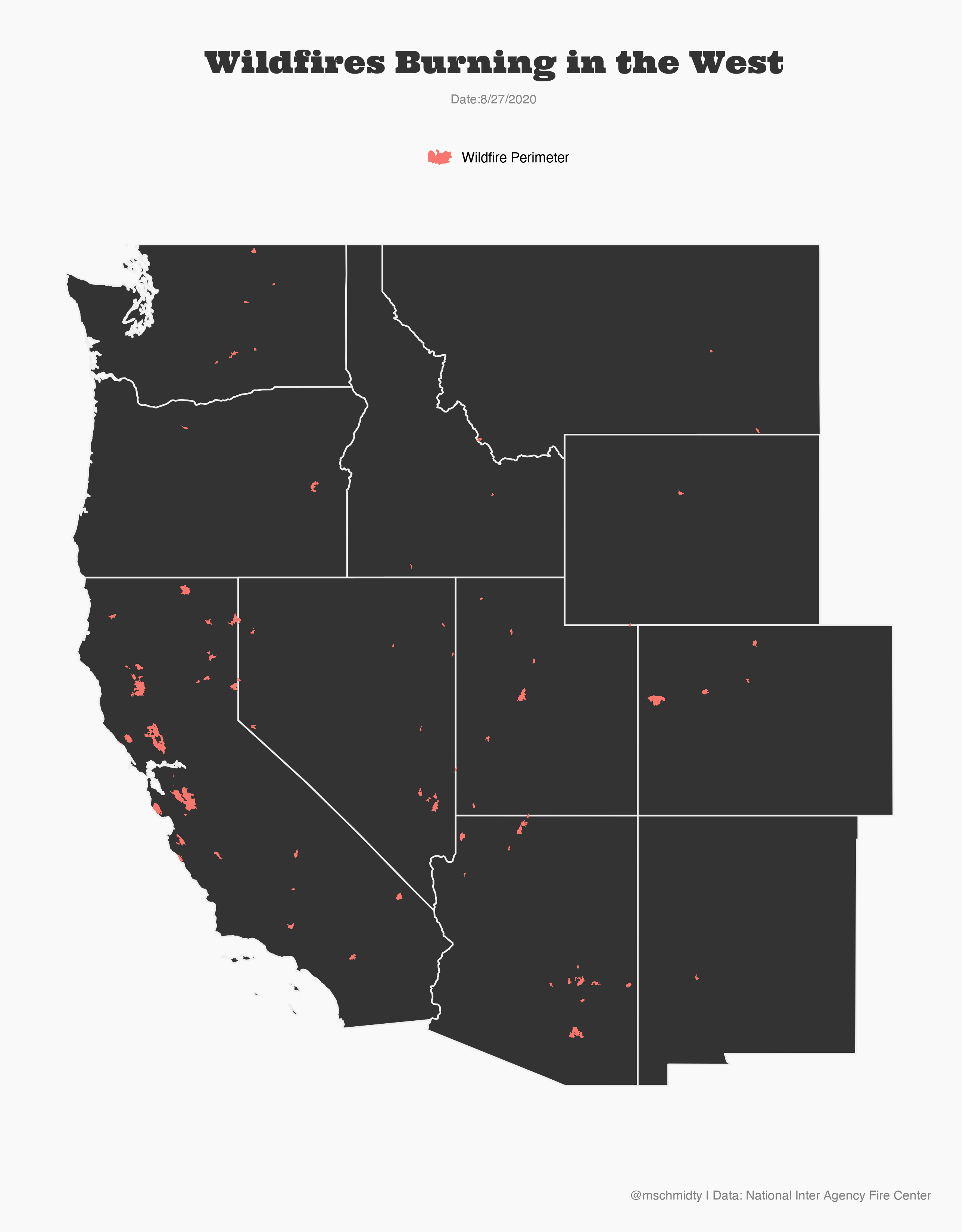
I wanted to see what that looks like on the landscape so I plotted all of the wildfires currently burning in the west. Surprisingly many fires are visible when plotted on a westwide scale.

It's pretty impressive to see how much of the west is currently burning or has burned this year. Even at a west wide scale the perimiters are still impressive.

R Scripts

library(tidyverse)
library(geojsonio)
library(sf)
library(rnaturalearth)
library(schmidtytheme)


theme_set(theme_schmidt()+
            theme(
              panel.grid.major = element_line(colour = "transparent")
            ))


wildfires<-geojson_read("https://opendata.arcgis.com/datasets/5da472c6d27b4b67970acc7b5044c862_0.geojson", what="sp")%>%
  st_as_sf()

usa <- ne_states(country="united states of america", returnclass="sf")

colorado<-usa%>%
  filter(name=="Colorado")

the_west<-usa%>%
  filter(name %in% c("California", "Oregon", "Washington", "New Mexico", "Arizona", "Nevada", "Idaho", "Wyoming","Montana", "Utah", "Colorado"))
  

ggplot()+
  geom_sf(data=the_west, fill="#333333", color="#efefef")+
  geom_sf(data = wildfires, fill="#FF6A5D", color=NA)+
  coord_sf(xlim = c(-125, -101), ylim = c(30, 50), expand = FALSE)+
  labs(
    title = "Wildfires Burning in the West",
    x="",
    y="",
    subtitle="Date:8/27/2020",
    caption="@mschmidty | Data: National Inter Agency Fire Center"
  )+
  theme(
    plot.background=element_rect(fill = "transparent", colour = NA),
    axis.text=element_blank(),
    panel.border=element_blank(),
    axis.line=element_blank(),
    plot.title=element_text(size=20)
  )+
  ggsave("Wildfires_in_the_west.png", h=11, w=11, type="cairo")

Fire Season totals

I also was curious to see how much fire activity has increased in the United States over time. I was particularly interested at looking at the year of the "Big Burn" in context to todays fire seasons.

I'm a bit scepticle of these numbers. I suspect that there is a bit of reporting bias in the data. Today there is a pipeline to report all fires. In the early 1900 I would guess that there were many fires that were not reported and that some of those that were reported were lost in the folders of history. Nonetheless it is still interesting to see how many more acres burn per year today than 50 and 100 years ago.

R Scripts

hist<-st_read(here("Dropbox", "r", "tidy_tuesday", "data", "InteragencyFirePerimeterHistory.shp"))

hist%>%
  as_tibble()%>%
  group_by(FIRE_YEAR)%>%
  summarize(total = sum(GIS_ACRES))%>%
  ungroup()%>%
  mutate(FIRE_YEAR = as.numeric(FIRE_YEAR))%>%
  filter(FIRE_YEAR>1900 & FIRE_YEAR!=9999 & FIRE_YEAR!=2050 & FIRE_YEAR!=2019)%>%
  ggplot(aes(FIRE_YEAR, total))+
  geom_segment( aes(x=FIRE_YEAR, xend=FIRE_YEAR, y=0, yend=total), color="grey30")+
  geom_point(size=3,  color="#FF6A5D", stroke = 1, fill=background_color, shape=21)+
  scale_x_continuous(breaks=c(1901,seq(1910, 2019, 10), 2018), expand = c(.01,0))+
  scale_y_continuous(labels = comma, expand = c(.01,0))+
  labs(
    title="Wildland Fire Acres Burned",
    subtitle="United States - 1901 to 2018",
    caption="@mschmidty | Data = National Interagency Fire Center",
    x = "", 
    y = "Total Acres Burned"
  )+
  annotate(
    geom = "curve", x = 1920, y = 4000000, xend = 1910.15, yend = 1700000 , 
    curvature = .3, arrow = arrow(length = unit(2, "mm"))
  )+
  annotate(geom = "text", 
           x = 1920, y = 4000000, 
           label = "1910 was the year of the Big Burn, \n a historic fire season that would \n drive Forest Service policy \n for generations to come", 
           hjust = "left",
           size=3)+
  theme(
    plot.background=element_rect(fill = "#f9f9f9", colour = NA),
    panel.grid=element_blank(),
    text=element_text(family="Public Sans"),
    plot.title=element_text(family="Ultra", size=30),
    axis.text = element_text(color = "gray40"),
    axis.text.x = element_text(margin = margin(1, 0, 20, 0)),
    axis.text.y = element_text(margin = margin(0,0,0,0))
  )

The Largest Fires in History

The last thing that I wanted to look at is the largest fires in US history. I used the package reactable for the first time to make a table of the 15 largest fires ever recorded.

As with many things in R, getting the reactable from R into HTML took quite a bit of hacking. I ended up exporting the table as HTML and adding it as an include in markdown.

R Scripts

library(reactable)

hist_area<-hist%>%
  st_area()

table_data<-hist%>%
  cbind(hist_area)%>%
  arrange(desc(hist_area))%>%
  head(17)%>%
  filter(LOCAL_NUM!="0020")%>%
  st_join(select(usa, woe_name))%>%
  as_tibble()%>%
  mutate(acres = as.numeric(hist_area)*0.000247105)%>%
  select(FIRE_YEAR, INCIDENT, acres, woe_name)%>%
  rename(Year=1, Name=2, Acres = 3, State = 4)%>%
  head(16)%>%
  filter(Name != "OKS - Starbuck" | State != "Oklahoma")%>%
  filter(Name != "Elk Mountain" | State != "Idaho")%>%
  filter(Name != "Wallow" | State != "Arizona")%>%
  mutate(State = case_when(
    Name == "Elk Mountain" ~ "Nevada & Idaho",
    Name == "OKS - Starbuck" ~ "Kansas & Oklahoma",
    Name == "Wallow" ~ "Arizona & New Mexico",
    TRUE ~ State
  ))%>%
  select(Name, Year, Acres, State)

bar_chart <- function(label, width = "100%", height = "14px", fill = "#00bfc4", background = NULL) {
  bar <- div(style = list(background = fill, width = width, height = height))
  chart <- div(style = list(flexGrow = 1, marginLeft = "6px", background = background), bar)
  div(style = list(display = "flex", alignItems = "center"), label, chart)
}

table_data%>%
  reactable(
    style = list(fontFamily="Public Sans", fontSize = 14),
    pagination = FALSE,
    defaultSorted = "Acres",
    theme = reactableTheme(
      headerStyle = list(
        fontFamily="Public Sans", 
        fontWeight = "bold"
      )
    ),
    columns = list(
      Name = colDef(
        style = list(fontFamily = "Public Sans", fontWeight = "bold")
      ),
      Acres = colDef(
        defaultSortOrder = "desc",
        cell = function(value) {
          width <- paste0(value * 100 / max(table_data$Acres), "%")
          value <- format(value, big.mark = ",")
          # Fix each label using the width of the widest number (incl. thousands separators)
          value <- format(value, width = 9, justify = "right")
          bar_chart(value, width = width, fill = "#3fc1c9")
        },
        align = "left",
        # Use the operating system's default monospace font, and
        # preserve white space to prevent it from being collapsed by default
        style = list(fontFamily = "monospace", whiteSpace = "pre")
      )
    )
  )