Will There be a Raftable Release out of McPhee Reservoir

February 09, 2020

tags:

I live next to the Dolores River. It’s an often overlooked gem of the southwest. It runs from just outside Rico, Colorado at its headwaters to the Colorado River near Moab, Utah. Rafting it is an experience.

As of late the river has become something of a destination for the rafting community. Most sections of the river are mellow and scenic. But two sections have class 4 rapids that keep things interesting: Snaggletooth Rapid and State Line Rapid (also known as the Chicken Raper Rapid).

In 1985 the McPhee Dam was completed, forever changing the flow of the lower Dolores River. Today, farmers, ranchers adn local ranchers rely on water from the McPhee Dam to to grow crops and raise livestock. As a result, the primary goal of reservoir managers is to keep as much water in the reservoir as possible. Raftable and ecological releases are secondary.This has resulted in several years where the reservoir has not filled and there have been no raftable releases. Other years reservoir managers say that the there will be no release and we get a release.

Because the Dolores is so loved in our community, there are a few people who try and predict when the Dolores will have a raftable release. Given my love of R, I thought it would be fun to do myself. The following are notes on how I built my model. I do my best to go over each step and detail why and how I included each covariate.

Load Packages

Here I load packages and set a custom theme. You can skip this part and just add in set_theme(theme_light) if you want to skip this part.

library(tidyverse) ## For all the data cleaning work.
library(lubridate) ## For working with dates.
library(extrafont) ## For Font Graphics
options(scipen = 999)

t<-theme_light()+
  theme(
    text=element_text(family = "Poppins", color = "#FFFFFF"),
    plot.margin = unit(c(0.5,0.5,0.5,0.5), "cm"),
    plot.title = element_text(face = "bold", size = rel(2.3), color = "#FFFFFF"),
    plot.subtitle = element_text(color = "#7A7A7A", size = rel(1.3), margin = margin(t = 0, r = 0, b = 15, l = 0)),
    plot.background = element_rect(fill = "#222222", color = "#FFFFFF"),
    panel.grid.major = element_line(color = "#555555"),
    panel.grid.minor = element_blank(),
    panel.background = element_rect(fill = "#222222", color = "#222222"),
    panel.border = element_blank(),
    axis.text = element_text(size = rel(0.8), colour = "#CCCCCC"),
    axis.title.x = element_text(margin = margin(t = 5, r = 0, b = 10, l = 0)),
    axis.title.y = element_text(margin = margin(t = 0, r = 10, b = 0, l = 20)),
    legend.title = element_text(face = "bold"),
    legend.text = element_text(color = "#222222"),
    legend.direction = "horizontal",
    legend.position="bottom",
    legend.key.width = unit(5, "cm"),
    legend.key.height = unit(0.3, "cm"),
    legend.box = "vertical",
    plot.caption = element_text(color = "#7A7A7A", size = rel(0.9))
  )
theme_set(t)

Getting a variable to predict

Getting Stream Guage Data Below McPhee Dam from the USGS

url<-paste0("https://waterservices.usgs.gov/nwis/dv/?format=rdb&sites=09169500,%2009166500&startDT=1985-02-01&endDT=", Sys.Date(), "&statCd=00003&siteType=ST&siteStatus=all")

flow_data<-read_tsv(url, skip = 35)%>%
  select(2:5)%>%
  rename(site_id = 1, date = 2, flow=3, code = 4)%>%
  mutate(site_id = ifelse(site_id == "09166500", "Dolores", "Bedrock"))%>%
  drop_na()

bedrock_flow<-flow_data%>%
  filter(site_id == "Bedrock"& year(date)>1986)%>%
  select(-code)

bedrock_flow

## # A tibble: 12,098 x 3
##    site_id date        flow
##    <chr>   <date>     <dbl>
##  1 Bedrock 1987-01-01   120
##  2 Bedrock 1987-01-02   130
##  3 Bedrock 1987-01-03   120
##  4 Bedrock 1987-01-04   120
##  5 Bedrock 1987-01-05   140
##  6 Bedrock 1987-01-06   140
##  7 Bedrock 1987-01-07   130
##  8 Bedrock 1987-01-08   130
##  9 Bedrock 1987-01-09   110
## 10 Bedrock 1987-01-10    95
## # … with 12,088 more rows

I want to predict the raftable days released below McPhee Dam. To do this I need flow data from a gauge below McPhee. Flow gauge data will tell me which days had enough flow to raft and which days did not. There are a few gauges to to choose from within the extensive USGS flow gauge system, but the oldest is at Bedrock, CO. To get the data I used the USGS Water Services REST API. There’s an R package that you can used to get the data, but since I’d used the API a few times before and I knew that the data could be returned in tab-separated format, I just used the readr::read_tsv() function.

Walk Through Notes:

The first step is to build the URL for the API. I used the USGS Rest API builder tool to get the right data.
Then used the read_tsv() function to pull data from the API skpping the first 35 lines of comments.
I then renamed the columns to something I could understand.
And then convert the site_ids to Characters instead of numbers. I pulled data from above and below the dams because at the time I thought I might use the data from above the Dam later for another predictive variable.
Then I drop all the missing values and subset the data to just below the dam.

Visualizing the flow

bedrock_flow%>%
  filter(year(date)>2007)%>%
  ggplot(aes(date, flow))+
  geom_line(color = "#1AB8FF", size =1.2, alpha = 0.6)+
  labs(title = "Dolores Flows from 2008 to Present",
       subtitle = "USGS Flow Gauge Site 09169500 Near Bedrock, Colorado",
       caption = "Data aquired from the Bureau of Reclemation using the RNRCS package.",
       y = "Flow Rate (cfs)",
       x = "Year")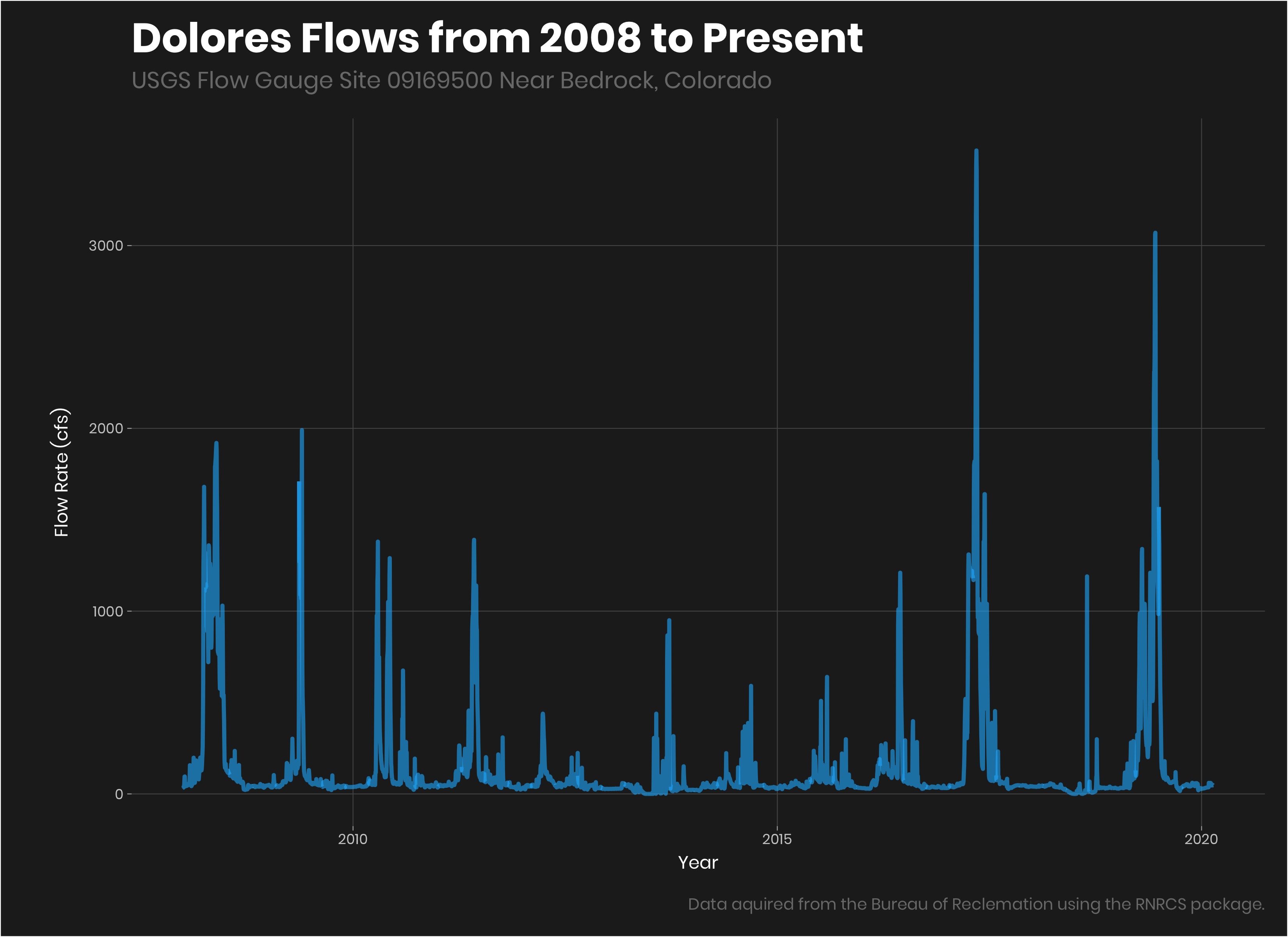

Subsetting the release

Next I needed to subset days where there is a raftable release. Releases happen during spring runoff so I wanted to subset those days in the spring that had greater than 800 cfs (cubic feet per second) of flow. I wanted to make sure to exclude non

predicted_variable<-bedrock_flow%>%
  filter(flow>800 & month(date) %in% c(3:7))%>%
  count(year(date))%>%
  rename(year = 1, raftable_releases = 2)

predicted_variable

## # A tibble: 21 x 2
##     year raftable_releases
##    <dbl>             <int>
##  1  1987                87
##  2  1988                13
##  3  1989                17
##  4  1991                 9
##  5  1992                61
##  6  1993                99
##  7  1994                35
##  8  1995                89
##  9  1997                82
## 10  1998                63
## # … with 11 more rows

Walk Through Notes:

First we filter the data for flows above 1000 cfs and dated from March to July (most of the monsoons occur from august to October).
Then we simply count the number of dates that are left by year.

We now have the variable we want to predict. Now we need predictors.

Getting the predictive variables.

There are many variables that affect reservoir volume. Current Reservoir volume and snowpack are probably two of the more important variables that are reliably measured. Snowpack tells us how much water will eventually be coming into the reservoir in the spring and reservoir volume tells us how much water is currently in the reservoir and also how much water we will need to cause a spill. Spring rain would be another variable that would be great to include, but I don’t want to rely on weather forecasts that far out. So we will stick with snowpack and current reservoir volume.

Snow Depth

The SNOTEL (Snow Telemetry) network provides snow data for 730 sites across the country. There are several in the Dolores watershed that can give us a bunch of data on snowpack. For this we will use the handy dandy package library(RNRCS) (the NRCS is the government agency in the Department of Agriculture that manages the SNOTEL network)

Finding All Snotel Sites in the Dolores Watershed

First we need to find which SNOTEL sites are within the Dolores River watershed to inform how much water could end up in McPhee reservoir.

library(RNRCS)
meta_data<-grabNRCS.meta(ntwrks = c("SNTL", "SNTLT", "SCAN"))

meta_data_unlist<-meta_data[[1]]%>%
  as_tibble()

meta_data_unlist

## # A tibble: 876 x 13
##    ntwk  wyear state site_name ts    start enddate latitude longitude
##    <chr> <fct> <fct> <chr>     <fct> <fct> <fct>   <fct>    <fct>    
##  1 SNTL  2019  AK    Frostbit… ""    2019… 2100-J… "  61.7… -149.27  
##  2 SNTL  2019  AK    McGrath   ""    2019… 2100-J… "  62.9… -155.61  
##  3 SNTL  2019  UT    Parleys … ""    2019… 2100-J… "  40.7… -111.61  
##  4 SNTL  2018  AK    East Pal… ""    2018… 2100-J… "  61.6… -149.10  
##  5 SNTL  2018  AK    Galena AK ""    2018… 2100-J… "  64.7… -156.71  
##  6 SNTL  2018  MT    JL Meadow ""    2017… 2100-J… "  44.7… -113.12  
##  7 SNTL  2018  NV    ONeil Cr… ""    2018… 2100-J… "  41.8… -115.08  
##  8 SNTL  2017  AK    Flower M… ""    2017… 2100-J… "  59.4… -136.28  
##  9 SNTL  2017  CA    Fredonye… ""    2016… 2100-J… "  40.6… -120.61  
## 10 SNTL  2017  UT    Bobs Hol… ""    2016… 2100-J… "  38.9… -112.15  
## # … with 866 more rows, and 4 more variables: elev_ft <fct>, county <fct>,
## #   huc <fct>, site_id <chr>

grabNRCS.meta - grabs all sites within the Snotel (“SNTL”), Snotel Lite, (“SNTLT”), and Scan (“SCAN”) systems. I’m really just interested in the snotel sites, but I wasn’t really sure what Snotel Lite or Scan was so I loaded them just in case. grabNRCS returns a single list, se we subset just the first item of the list.

dolores_sites<-meta_data_unlist%>%
  filter(state =="CO", str_detect(huc, "140300"))%>%
  mutate(site_id_num = as.numeric(str_match_all(site_id, "[0-9]+")))

dolores_sites

## # A tibble: 6 x 14
##   ntwk  wyear state site_name ts    start enddate latitude longitude
##   <chr> <fct> <fct> <chr>     <fct> <fct> <fct>   <fct>    <fct>    
## 1 SNTL  2011  CO    Black Me… ""    2011… 2100-J… "  37.7… -108.18  
## 2 SNTL  2005  CO    Sharksto… ""    2004… 2100-J… "  37.5… -108.11  
## 3 SNTL  1986  CO    El Dient… ""    1985… 2100-J… "  37.7… -108.02  
## 4 SNTL  1986  CO    Scotch C… ""    1985… 2100-J… "  37.6… -108.01  
## 5 SNTL  1980  CO    Lizard H… ""    1979… 2100-J… "  37.8… -107.92  
## 6 SNTL  1980  CO    Lone Cone ""    1979… 2100-J… "  37.8… -108.20  
## # … with 5 more variables: elev_ft <fct>, county <fct>, huc <fct>,
## #   site_id <chr>, site_id_num <dbl>

dolores_sites - We then filter all sites in Colorado (“CO”) and detect all of the huc values with 140300. To pull data from the sites we will need a site ID number. The Meta data has the site IDs in a string that contains characters and numbers.

dolores_site_ids<-dolores_sites%>%
  pull(site_id_num)%>%
  unlist()%>%
  as.numeric()

dolores_site_ids

## [1] 1185 1060  465  739  586  589

dolores_site_ids - The last step is to convert the site_id_num variable into a vector so that we can pull data from each site in the next step.

Pulling the data from the snotel sites

Function to Pull All Sites

First we need a function that we can loop over each of the snotel site IDs and pull data for each of one. grabNRCS.data does not allow you to pull data from more than one site at a time.

get_snotl_data<-function(site_id){
  grabNRCS.data(network = "SNTL",
              site_id = site_id,
              timescale = "daily",
              DayBgn = '1985-01-01',
              DayEnd = Sys.Date()
              )%>%
    as_tibble()%>%
    mutate(site_id_num = site_id)
}

To get data from each site we need to use grabNRCS.data() function. grabNRCS.data takes:

network - the network we want to pull from.
the site_id which we produced a list of in the last step.
DayBgn - The first day you want to pull data from.
DayEnd - the Last date you want data from. Here we use the system data (Today).

We then convert the data to a tibble for better output in Rstudio and add a column with mutate with the site_id number for working with the data later.

Getting ALL the data with lapply

all_sntl_data<-lapply(dolores_site_ids, get_snotl_data)%>%
  bind_rows()

all_sntl_data

## # A tibble: 58,531 x 22
##    Date  Air.Temperature… Air.Temperature… Air.Temperature…
##    <chr>            <int>            <int>            <int>
##  1 2012…               46               52               42
##  2 2012…               46               53               42
##  3 2012…               52               62               44
##  4 2012…               52               61               46
##  5 2012…               52               64               46
##  6 2012…               54               64               47
##  7 2012…               53               64               49
##  8 2012…               52               61               47
##  9 2012…               54               63               49
## 10 2012…               50               61               42
## # … with 58,521 more rows, and 18 more variables:
## #   Air.Temperature.Observed..degF..Start.of.Day.Values <int>,
## #   Precipitation.Accumulation..in..Start.of.Day.Values <dbl>,
## #   Snow.Depth..in..Start.of.Day.Values <int>,
## #   Snow.Water.Equivalent..in..Start.of.Day.Values <dbl>,
## #   Soil.Moisture.Percent..4in..pct..Start.of.Day.Values <dbl>,
## #   Soil.Moisture.Percent..8in..pct..Start.of.Day.Values <dbl>,
## #   Soil.Moisture.Percent..20in..pct..Start.of.Day.Values <dbl>,
## #   Soil.Moisture.Percent..40in..pct..Start.of.Day.Values <dbl>,
## #   Soil.Temperature.Observed..4in..degF..Start.of.Day.Values <int>,
## #   Soil.Temperature.Observed..8in..degF..Start.of.Day.Values <int>,
## #   Soil.Temperature.Observed..20in..degF..Start.of.Day.Values <int>,
## #   Soil.Temperature.Observed..40in..degF..Start.of.Day.Values <int>,
## #   site_id_num <dbl>,
## #   Soil.Moisture.Percent..2in..pct..Start.of.Day.Values <dbl>,
## #   Soil.Temperature.Observed..2in..degF..Start.of.Day.Values <int>,
## #   Wind.Direction.Average..degree. <int>, Wind.Speed.Average..mph. <dbl>,
## #   Wind.Speed.Maximum..mph. <dbl>

lapply takes:

dolores_site_ids a vector of values to loop over.
get_snotl_data a function to inject each of the vector values into one at a time.

lapply returns a list so the final step is to bind_rows which merges all of the columns.

Cleaning the Data

I’m going to predict number of days the Dolores Runs in a year, so I need to convert the snow data from daily data from multiple sites to annual data from all sites. I’m assuming that max snow water equivalant correlates best with runoff in this dataset so we will use that to summarize each year.

se_site<-all_sntl_data%>%
  select(Date, Snow.Depth..in..Start.of.Day.Values, Snow.Water.Equivalent..in..Start.of.Day.Values, site_id_num)%>%
  mutate(
    date = as.Date(Date)
    )%>%
  rename(snow_depth = 2, snow_water_eq=3)%>%
  filter(site_id_num %in% c(465, 586, 589, 739))

se_site

## # A tibble: 50,182 x 5
##    Date       snow_depth snow_water_eq site_id_num date      
##    <chr>           <int>         <dbl>       <dbl> <date>    
##  1 1986-08-05         NA            NA         465 1986-08-05
##  2 1986-08-06         NA             0         465 1986-08-06
##  3 1986-08-07         NA             0         465 1986-08-07
##  4 1986-08-08         NA             0         465 1986-08-08
##  5 1986-08-09         NA             0         465 1986-08-09
##  6 1986-08-10         NA             0         465 1986-08-10
##  7 1986-08-11         NA             0         465 1986-08-11
##  8 1986-08-12         NA             0         465 1986-08-12
##  9 1986-08-13         NA             0         465 1986-08-13
## 10 1986-08-14         NA             0         465 1986-08-14
## # … with 50,172 more rows

First we select the columns that contain the Date, Snow Depth and Snow water Equivalant. I don’t end up using Snow depth because it only goes back to around 2000 for all sites while snow water equivalant goes back to 1986.
mutate add a date field that is formatted as a date.
rename snow depth and snow water equivalant to something more manageable.
The last thing we do is subset the sites to only those that have been around since 1986 using filter.

Let’s take a look at these sites really quick to see how they look.

se_site%>%
  filter(year(date)>2007)%>%
  ggplot(aes(date, snow_water_eq, color = as.factor(site_id_num)))+
  geom_line(size = 1.5, alpha = 0.5)+
  theme_light()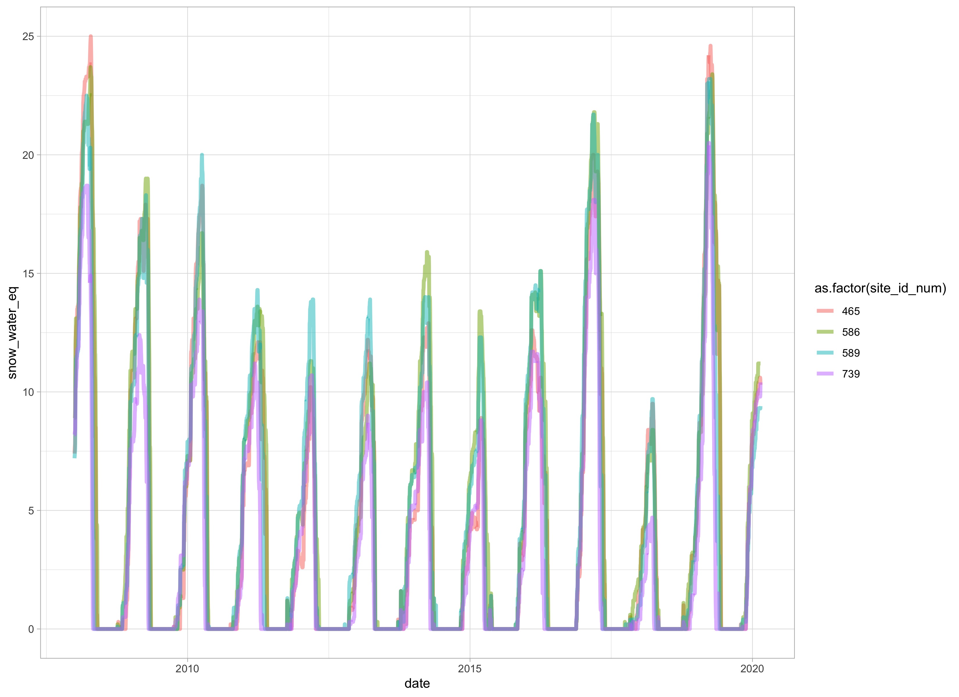

se_site_year<-se_site%>%
  group_by(year(date), site_id_num)%>%
  summarize(max_se = max(snow_water_eq, na.rm = T))%>%
  ungroup()%>%
  rename(year=1)

se_site_year

## # A tibble: 142 x 3
##     year site_id_num max_se
##    <dbl>       <dbl>  <dbl>
##  1  1985         586   21.6
##  2  1985         589   23.5
##  3  1986         465    6.3
##  4  1986         586   19.8
##  5  1986         589   20.8
##  6  1986         739    5.1
##  7  1987         465   19.1
##  8  1987         586   19.1
##  9  1987         589   22  
## 10  1987         739   20.1
## # … with 132 more rows

The next several steps are where the sausage is made. First I want the max value for snow water equivalant for each site per year. To do this, we group_by year(date) which uses the date field to group the data and then. We also want to group by site_id_num so we add that to the group_by as well.
We can then summarize by our groups. Here we want to make a variable caleed max_se which is the max of the snow_water_eq field within the group we described above.
Lastly we ungroup the data (group_by can cause nasty problems if not ungrouped) and rename the year(date) column to year.

Combining a subset of sites

To simplify things we will average the sites. I think if I did this again I would not average the sites but have each site be a predictor.

avg_snwater_eq<-se_site_year%>%
  filter(year>1986)%>%
  group_by(year)%>%
  summarize(avg_snow_water_e = mean(max_se))%>%
  ungroup()

avg_snwater_eq

## # A tibble: 34 x 2
##     year avg_snow_water_e
##    <dbl>            <dbl>
##  1  1987            20.1
##  2  1988            11.4
##  3  1989            16.3
##  4  1990             9.28
##  5  1991            16.5
##  6  1992            15.5
##  7  1993            25.4
##  8  1994            12.3
##  9  1995            21.8
## 10  1996            13.6
## # … with 24 more rows

Only 4 of the 6 sites in the basin have values all the way back to 1986, the year that the McPhee Dam was put in.
We then group_by year because we want one value per year.
Then summarize the max snow water equivalent (max_se) - created in the last step - as a mean of the four site maxes per year.
And then, as always, ungroup.

Summary of Snotel Snow depth

Now we have our first predictive variable: average max snow water equivalent four three snotel sites in the Dolores River watershed.

The steps we took to get that data: 1. We used the RNRCS package to… 2. Get all sites in the Snotel Network with grabNRCS.meta() 3. We then subset those sites to just those in the Dolores watershed. 4. We then used the site_ids to get daily snow data from each site. 5. We combined each sites data into one dataframe. 6. We then grouped the data to get the max snow water equivalent for each site for each year. 7. We then averaged the maxes from four sites to get one average snow water equivalent per year.

Prediction of Future Snowpack

We’ll use the {fable} package for timeseries forecasting.

library(fable) #For prediction

For forecasting we need an average of all four sites per day. We want to predict what the average will be.

avg_sn<-se_site%>%
  filter(year(Date)>1987)%>%
  group_by(Date)%>%
  summarize(avg_sn_eq =  mean(snow_water_eq, rm.na = T))%>%
  ungroup()%>%
  mutate(Date = as.Date(Date))


avg_sn

## # A tibble: 11,741 x 2
##    Date       avg_sn_eq
##    <date>         <dbl>
##  1 1988-01-01      4.1
##  2 1988-01-02      4.18
##  3 1988-01-03      4.38
##  4 1988-01-04      4.53
##  5 1988-01-05      4.82
##  6 1988-01-06      5.4
##  7 1988-01-07      5.6
##  8 1988-01-08      5.65
##  9 1988-01-09      5.8
## 10 1988-01-10      5.9
## # … with 11,731 more rows

We filter years after 1987 because we don’t want the year that they were filling the reservior to influence the prediction.
Next we group by Date which is daily and then summarize, averaging all four sites for that day. We ungroup to prevent weird stuff from happening.
And lastly we convert the Date column, which for some reaon was converted to a character, to an actual date with as.Date.

Let see what it looks like:

avg_sn%>%
  ggplot(aes(Date, avg_sn_eq))+
  geom_line(color = "#1AB8FF", size = 2, alpha = 0.5)+
  labs(title = "Average Snow Water Equivalant",
       subtitle = "From four Snotel Sites in the Dolores River watershed",
       y = "Avg. Snow Water Equivalant")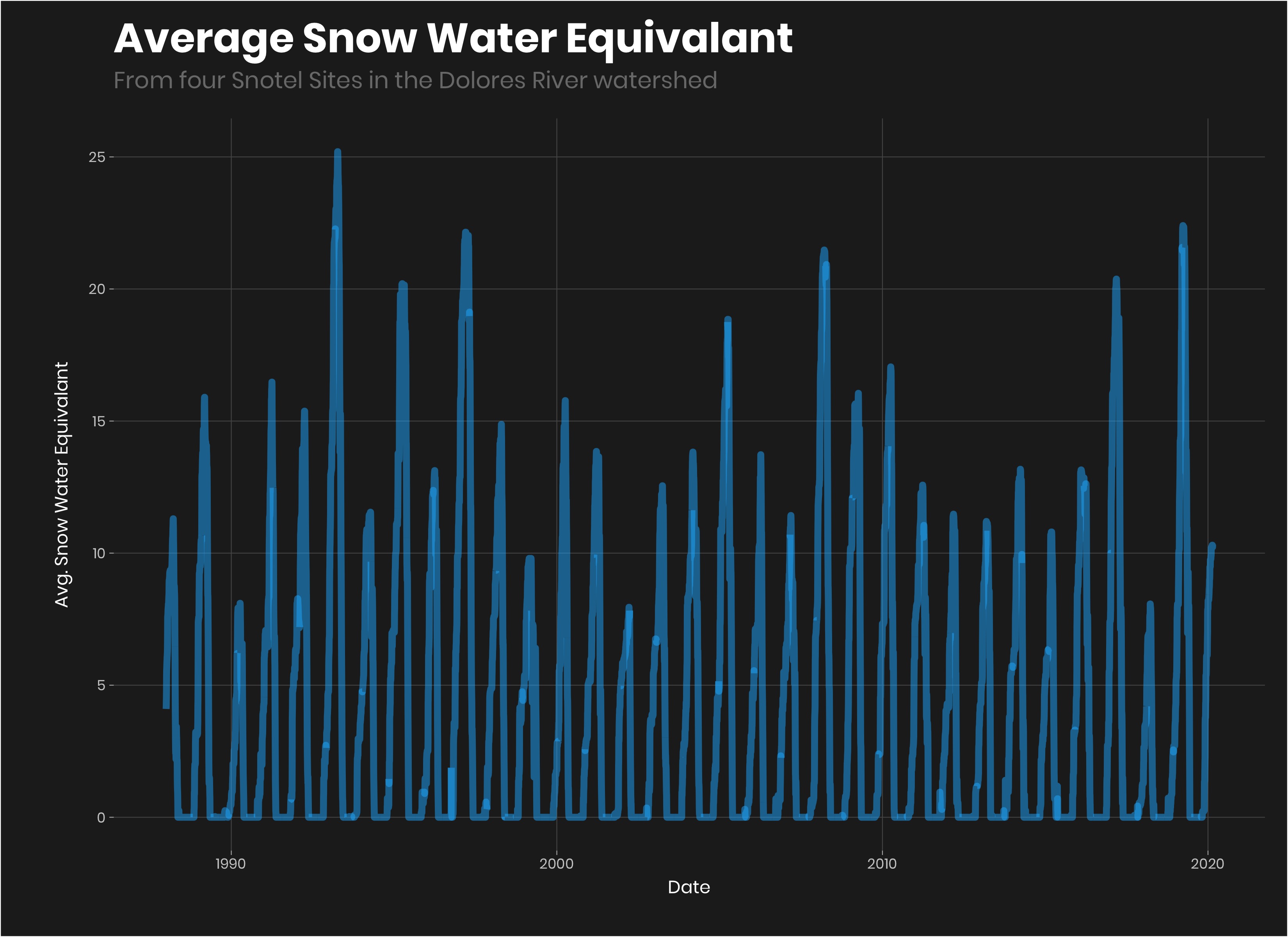

Average Snow Water Equivalant in Dolores Watershed, 1986 to present

To do a timeseries forcast we need to convert the data into tsibble format. I don’t know a ton about tsibbles. I think they are basically just a tibble with an time index.

avg_sn_ts<-avg_sn%>%
  as_tsibble(index = Date)

Next we will make our model. I by no means am an expert at forecasting (this took me an embarassingly long time). Many of my initial tries failed using a variety of other models. I finally got an auto ARIMA forecast to work using fourier. If you want to learn more about forecasting, check out Rob Hyndman’s Blog.

fit<-avg_sn_ts%>%
  model(
    arima = ARIMA(avg_sn_eq~fourier("year", K = 15))
  )

fit%>%
  forecast(h = "3 months")%>%
  autoplot(avg_sn_ts%>%filter(year(Date)>2018))+
  geom_line(color = "#ffffff", size = 2)+
  labs(title = "Snowpack Prediction",
       subtitle = "Dolores River watershed Snotel sites",
       y = "Avg. Snow Whater Equivalant")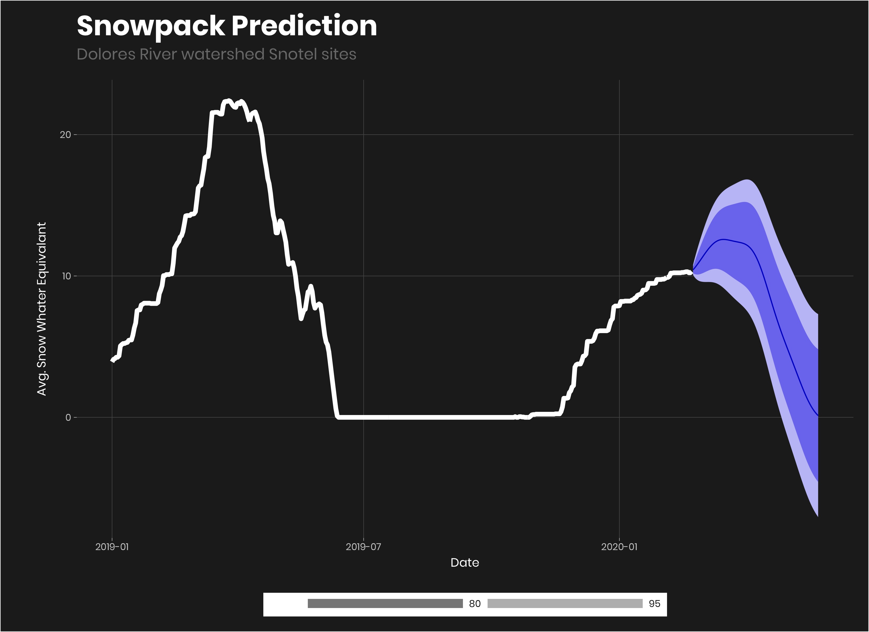

Snow water equivalant forecast for the next six months.

Looking at the forecast in the autoplot() which is just an easy ggplot for forecasting, it looks to me that the forecast looks pretty good, but might be a bit optimistic for the average. But it’s hard to tell. We could get a lot of snow in the end of February or March. It gives us a good range to work with and use in our predictions.

To use in our prediction we need a max, min and average value for the max snowpack.

pred_sn_pk<-fit%>%
  forecast(h = "6 months")%>%
  filter(avg_sn_eq == max(avg_sn_eq))%>%
  mutate(ci_90 = hilo(.distribution, 90))%>%
  mutate(pred_lower = ci_90$.lower, pred_upper = ci_90$.upper)%>%
  as_tibble()%>%
  rename(pred_avg_sn_eq = avg_sn_eq)%>%
  select(Date, pred_avg_sn_eq, pred_lower, pred_upper)%>%
  pivot_longer(-Date, names_to = "estimated_eq", values_to = "avg_snow_water_e")%>%
  mutate(year = year(Date))%>%
  select(-Date)

pred_sn_pk

## # A tibble: 3 x 3
##   estimated_eq   avg_snow_water_e  year
##   <chr>                     <dbl> <dbl>
## 1 pred_avg_sn_eq            12.6   2020
## 2 pred_lower                 9.70  2020
## 3 pred_upper                15.5   2020

Use our model to forecast() six months out.
filter out the max value for the average (this isn’t perfect but it will work for our purposes).
Add a column with higher and lower values based on a 90% confidence interval using the hilo function.
convert to a tibble.
Select only the values we want.
pivot_longer so that we have a year column and a snow_water_equivalant column.
Make a year column.
drop the Date column.

Reservoir Volume

The next variable we need is reservoir volume. ### Get Daily McPhee Reservoir Volumes

bor_data<-grabBOR.data(site_id = "MPHC2000",
                       timescale = 'daily',
                       DayBgn = '1985-01-01',
                      DayEnd = Sys.Date())%>%
  as_tibble()%>%
  mutate(date = as.Date(Date),
         res_volume = as.numeric(`Reservoir Storage Volume (ac_ft) Start of Day Values`))%>%
  select(date, res_volume)

bor_data

## # A tibble: 12,826 x 2
##    date       res_volume
##    <date>          <dbl>
##  1 1985-01-01      44997
##  2 1985-01-02      45079
##  3 1985-01-03      45161
##  4 1985-01-04      45189
##  5 1985-01-05      45207
##  6 1985-01-06      45262
##  7 1985-01-07      45372
##  8 1985-01-08      45463
##  9 1985-01-09      45601
## 10 1985-01-10      45721
## # … with 12,816 more rows

We use the {RNRCS} package again to get Bureau of Reclemation (BOR - the agency that managed the McPhee dam)data.

The {RNRCS} package has a function to grab Bureau of Reclemation data grabBOR.data(). It works much the same way as the grapNRCS.data() function that we wrapped our own function around above. However this time, we only needed one site so I just looked it up and put it in instead of using a meta function to get sites like we did with the snotel data.
We convert the data to a tibble (df) convert the date to date format and convert the volume into numeric.
We then subset the columns to just date and reservoir volume.

Summarize data to yearly

res_vol<-bor_data%>%
  filter(month(date) %in% c(01, 02))%>%
  group_by(year(date))%>%
  summarize(min_vol = min(res_volume, na.rm = T))%>%
  ungroup()%>%
  rename(year = 1)%>%
  filter(year>1986)

res_vol

## # A tibble: 34 x 2
##     year min_vol
##    <dbl>   <dbl>
##  1  1987  293309
##  2  1988  324234
##  3  1989  319239
##  4  1990  274597
##  5  1991  241536
##  6  1992  297471
##  7  1993  304632
##  8  1994  310609
##  9  1995  268308
## 10  1996  312568
## # … with 24 more rows

Here we subset the data to just the winter months and then summarize by year by getting the minimum value for all three months (I originally averaged the months, but getting the min gives a better prediction).

First we filter January and February to get that years lowest reservoir values prior to runoff.
We then group_by() year and then get the minimul volume from each of the two months.
then we rename the first column to year instead of year(date) and filter out all years before 1987.

Building the Model

Combining the variables and the datasets.

var_df<-predicted_variable%>%
  full_join(avg_snwater_eq)%>%
  full_join(res_vol)%>%
  arrange(year)%>%
  mutate(raftable_releases = ifelse(is.na(raftable_releases), 0, raftable_releases))

var_df_train<-var_df%>%
  filter(year!=2020)

var_df_test<-var_df%>%
  filter(year==2020)

var_df_train

## # A tibble: 33 x 4
##     year raftable_releases avg_snow_water_e min_vol
##    <dbl>             <dbl>            <dbl>   <dbl>
##  1  1987                87            20.1   293309
##  2  1988                13            11.4   324234
##  3  1989                17            16.3   319239
##  4  1990                 0             9.28  274597
##  5  1991                 9            16.5   241536
##  6  1992                61            15.5   297471
##  7  1993                99            25.4   304632
##  8  1994                35            12.3   310609
##  9  1995                89            21.8   268308
## 10  1996                 0            13.6   312568
## # … with 23 more rows

To join the datasets we use a full join because not every year has a raftable release and therefore has some year missing. Both of the other datasets have data for each year and a full join fills any missing variables with NA but keeps all observations.
The years with NA values for raftable release should be 0, because those are the years without a raftable release and we want to th model to predict when those years are as well.
Lastly we make two datasets one to train the model, which includes all years except this year 2020, and test model this year.

Note: typically you want to split the data into training and testing datasets so you can train your model with the training dataset and then evaluate it with the testing dataset that it hasn’t seen. But here we don’t really care that much because this is just fun and we can predict this upcoming release and see if it is right.

Random Forest Using `caret`

library(caret)
set.seed(1234)

control <- trainControl(method="cv", number=10)

rf_model <- train(raftable_releases~avg_snow_water_e+min_vol,
                    data=var_df_train,
                    method="rf",
                    tuneLength=3,
                    trControl=control)

## note: only 1 unique complexity parameters in default grid. Truncating the grid to 1 .

rf_model

## Random Forest
##
## 33 samples
##  2 predictor
##
## No pre-processing
## Resampling: Cross-Validated (10 fold)
## Summary of sample sizes: 29, 31, 29, 29, 29, 30, ...
## Resampling results:
##
##   RMSE      Rsquared   MAE     
##   15.69357  0.6885501  13.05262
##
## Tuning parameter 'mtry' was held constant at a value of 2

Here we build a cross validated random forest regression model to go predict number of raftable days.

meothod = "repeatedcv" is repeated cross validation where we do 10 cross validations 3 times with a random search.
We use the train() functio from caret to fit the model using both predictive variables avg_snow_water_e and min_vol.
We use Random Forest algorythm "rf" with 2000 trees.
we try 3 mtry depths (thgere are only two because we have only two variables, but tuneLength of two was not tuning at all for some reason).

Evaluating the model

WARNING: this is not how you should evaluate a model typically like I said above.

var_df_train%>%
  mutate(prediction = stats::predict(rf_model, .))%>%
  ggplot(aes(raftable_releases, prediction))+
  geom_point(color = "#1AB8FF", size =4, alpha = 0.6)+
  geom_text(aes(label=year),hjust=-0.3, vjust=-0.3, color = "#FFFFFF")+
  labs(title = "Random Forest: Predicted vs Actual Raftable Release Days",
       x = "Actual Release Days",
       y = "Predicted Release Days",
       subtitle = "Sudo-testing accuracy of RF model")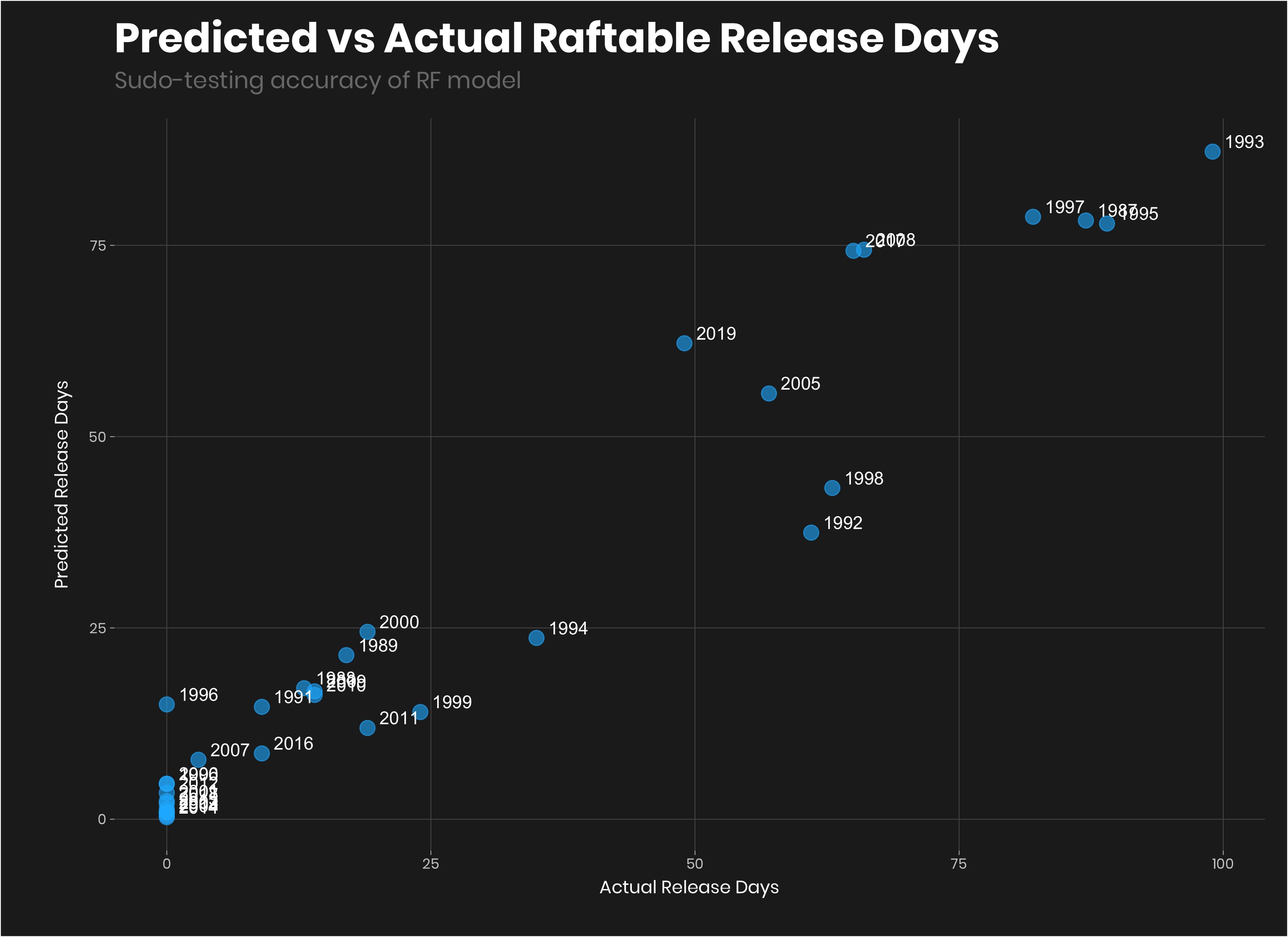

Predicted vs Actual Raftable Release Days

Pretty good. Again, I keep saying this becuase it is really important, we would want to make sure that the model works in out of training sample, but with this dataset, we don’t have enough data to do that.

So what about this year

var_df_test%>%
  mutate(prediction = predict(rf_model, .))

## # A tibble: 1 x 5
##    year raftable_releases avg_snow_water_e min_vol prediction
##   <dbl>             <dbl>            <dbl>   <dbl>      <dbl>
## 1  2020                 0             10.4  287807       4.71

So far the model predicts we will have 4.7078333 days of raftable flows. I’d say that is within the margin of error of 0 days looking at past predictions. But what if we get more snow? Given that it is February and Peak snow is typically around mid March would be a good assumption.

Let’s add the snotel forcast from the ARIMA model above to the predicted dataset.

pred_sn_pk_1<-pred_sn_pk%>%
  mutate(min_vol = var_df%>%
           filter(year == 2020)%>%
           pull(min_vol))

test_data<-var_df%>%
  filter(year==2020)%>%
  select(-raftable_releases)%>%
  mutate(estimated_eq = "current")%>%
  bind_rows(pred_sn_pk_1)

test_data

## # A tibble: 4 x 4
##    year avg_snow_water_e min_vol estimated_eq  
##   <dbl>            <dbl>   <dbl> <chr>         
## 1  2020            10.4   287807 current       
## 2  2020            12.6   287807 pred_avg_sn_eq
## 3  2020             9.70  287807 pred_lower    
## 4  2020            15.5   287807 pred_upper

Now let’s use the prediction for current, pred_avg_sn_eq, pred_lower, and pred_upper

test_data%>%
  mutate(prediction = stats::predict(rf_model, .))

## # A tibble: 4 x 5
##    year avg_snow_water_e min_vol estimated_eq   prediction
##   <dbl>            <dbl>   <dbl> <chr>               <dbl>
## 1  2020            10.4   287807 current              4.71
## 2  2020            12.6   287807 pred_avg_sn_eq       6.60
## 3  2020             9.70  287807 pred_lower           3.09
## 4  2020            15.5   287807 pred_upper          23.0

That looks pretty good.

Current Prediction is 4.71 days.
Predicted is 6.6 at the average forecast snowdepth.
3.09 is the low end. And 23 days if we get dumped on from now until April 1.

Let’s try something a bit simpler, like a linear model.

model_lm<-glm(raftable_releases~avg_snow_water_e+min_vol, family = "poisson", data = var_df_train)

##saveRDS(model_lm, "output/models/lm_model.rds")

summary(model_lm)

##
## Call:
## glm(formula = raftable_releases ~ avg_snow_water_e + min_vol,
##     family = "poisson", data = var_df_train)
##
## Deviance Residuals:
##    Min      1Q  Median      3Q     Max  
## -6.033  -3.211  -2.308   1.997   6.488  
##
## Coefficients:
##                       Estimate    Std. Error z value             Pr(>|z|)
## (Intercept)      -2.0553926585  0.2693758160   -7.63   0.0000000000000234
## avg_snow_water_e  0.1900049675  0.0072692190   26.14 < 0.0000000000000002
## min_vol           0.0000076058  0.0000008358    9.10 < 0.0000000000000002
##                     
## (Intercept)      ***
## avg_snow_water_e ***
## min_vol          ***
## ---
## Signif. codes:  0 '***' 0.001 '**' 0.01 '*' 0.05 '.' 0.1 ' ' 1
##
## (Dispersion parameter for poisson family taken to be 1)
##
##     Null deviance: 1292.88  on 32  degrees of freedom
## Residual deviance:  446.98  on 30  degrees of freedom
## AIC: 563.07
##
## Number of Fisher Scoring iterations: 6

This model looks pretty good.

model_lm%>%
  augment(data = var_df_train, type.predict = "response")%>%
  ggplot(aes(raftable_releases, .fitted))+
  geom_point(color = "#1AB8FF", size =4, alpha = 0.6)+
  geom_text(aes(label=year),hjust=-0.3, vjust=-0.3, color = "#FFFFFF")+
  labs(title = "Linear Model: Predicted vs Actual Raftable Release Days",
       subtitle = "Actual Values vs. Predicted Values",
       y = "Predicted Values",
       x = "Actual Raftable Release Days")

Linear Model: Predicted vs Actual Raftable Release Days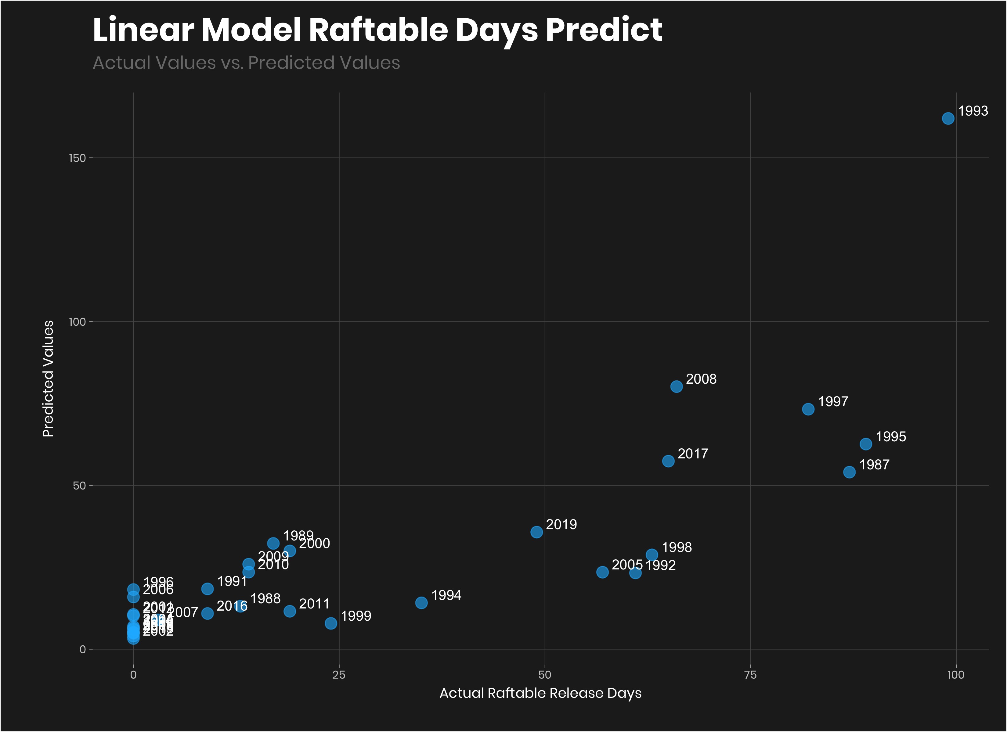

model_lm%>%
  augment(newdata = test_data, type.predict = "response")

## # A tibble: 4 x 6
##    year avg_snow_water_e min_vol estimated_eq   .fitted .se.fit
##   <dbl>            <dbl>   <dbl> <chr>            <dbl>   <dbl>
## 1  2020            10.4   287807 current           8.25   0.620
## 2  2020            12.6   287807 pred_avg_sn_eq   12.5    0.767
## 3  2020             9.70  287807 pred_lower        7.21   0.575
## 4  2020            15.5   287807 pred_upper       21.6    0.986

That looks more rational than the random forest model. The results:

Current snowpack = 8.25 days
predicted peak snowpack = 12.5 days.
predicted lower snowpack = 7.21 (this really isn’t rational considering current is already greater than it).
predicted upper snowpack = 21.6 days (let it snow let it snow).

I’ll continue to run this as the winter progresses. We now have a model that we can push into production to predict future data sets.