Colorado: Hex Plots, API packages, and R
I've been seeing a lot of hex plots made with r. They are a way to semi-artistically visualize spatial data. Although I don't think this is completely appropriate for most visualizations, it looks amazing. Here are a few examples of how I made hex plots in R.
I used a lot of packages for this. Most of them are used to get data. Only sf, raster, tidyverse and viridis will be used to wrangle and plot the spatial data.
library(prism)
library(tidyverse)
library(raster) ## Raster spatial data
library(sf) ## Vector spatial data
library(viridis) ## Color Scheme
library(tidycensus) ## Getting Census Data
library(tigris) ## Getting state and census boundary shapefiles
library(extrafont) ## Better fonts for graphs
library(elevatr) ## Getting elevation data
library(osmdata) ## Open street map data

##font_import()  ## Load all the fonts. You only need to do this once.

fonttable()%>%
  View()  ## Allows you to view all of the available fonts.
First a little custom styling for the theme_void theme.
t<-theme_void()+
  theme(
    text=element_text(family = "Playfair Display"),
    plot.margin = unit(c(1,1,1,1), "cm"),
    plot.title = element_text(face = "bold", size = 22, hjust = 0.5, color = "#222222"),
    plot.subtitle = element_text(hjust = 0.5, color = "#7A7A7A", size = 15),
    plot.background = element_rect(fill = "#f9f9f9", color = "#f9f9f9"),
    panel.grid.major = element_line(color = "#f9f9f9"),
    panel.grid.minor = element_blank(),
    legend.title = element_text(face = "bold"),
    legend.text = element_text(color = "#7A7A7A"),
    legend.direction = "horizontal",
    legend.position="bottom",
    legend.key.width = unit(5, "cm"),
    legend.key.height = unit(0.3, "cm"),
    legend.box = "vertical"
  )
theme_set(t)
Total precipitation
Download the data using prism package from the University of Oregon PRISM climate dataset. YOU ONLY NEED TO DO THIS ONCE and the normals will be saved to a folder on your coputer in this case I saved them to "data/prism"!
options(prism.path = "data/prism") ## set the path to download the data
get_prism_normals("ppt", "800m", mon = c(1:12), keepZip = TRUE) ## download the data (downlaoding all months and keeping the zip files.)
Next wee need to read all of the each raster we just downloaded and then stack those into a rasterBrick object.
file_paths<-ls_prism_data(absPath = T)[1:12,2] ## List all file paths.  Make sure the run the option(prism.path = "data/prism") before running this.
list_rasters<-lapply(file_paths, raster) ## use list of file paths to read each one with function raster.

names<-c("January", "February", "March", "April", "May", "June", "July", "August", "September", "October", "November", "December" )
names(list_rasters)<-names ## rename each list item to it's corresponding month.

(data<-brick(list_rasters)) ## Combine into a brick. This takes some time.
Subsetting the Raster and Readying the Hexagons
PRISM data covers the entire united states. I only want to look at precipitation data for Colorado so we need to subset the data. To get the shapefile for the state of Colorado we can use an the amazing tigris package. We will then need to crop the raster to the state of Colorado. The last step will be to extract the data to a hexagonal shapefile.
state_shape<-counties("Colorado") ## Get county shape

data_cropped_state<-data%>%
  crop(state_shape) ## Crop the raster data by the county shape
Now we make a hex grid that we are going to extract the raster data into. To do this we use the sf::st_make_grid function.
(state_grid<-state_shape%>%
  st_as_sf()%>%
  st_make_grid(cellsize = .1,
               square = FALSE))

state_grid%>%
ggplot()+
  geom_sf(fill = "white")
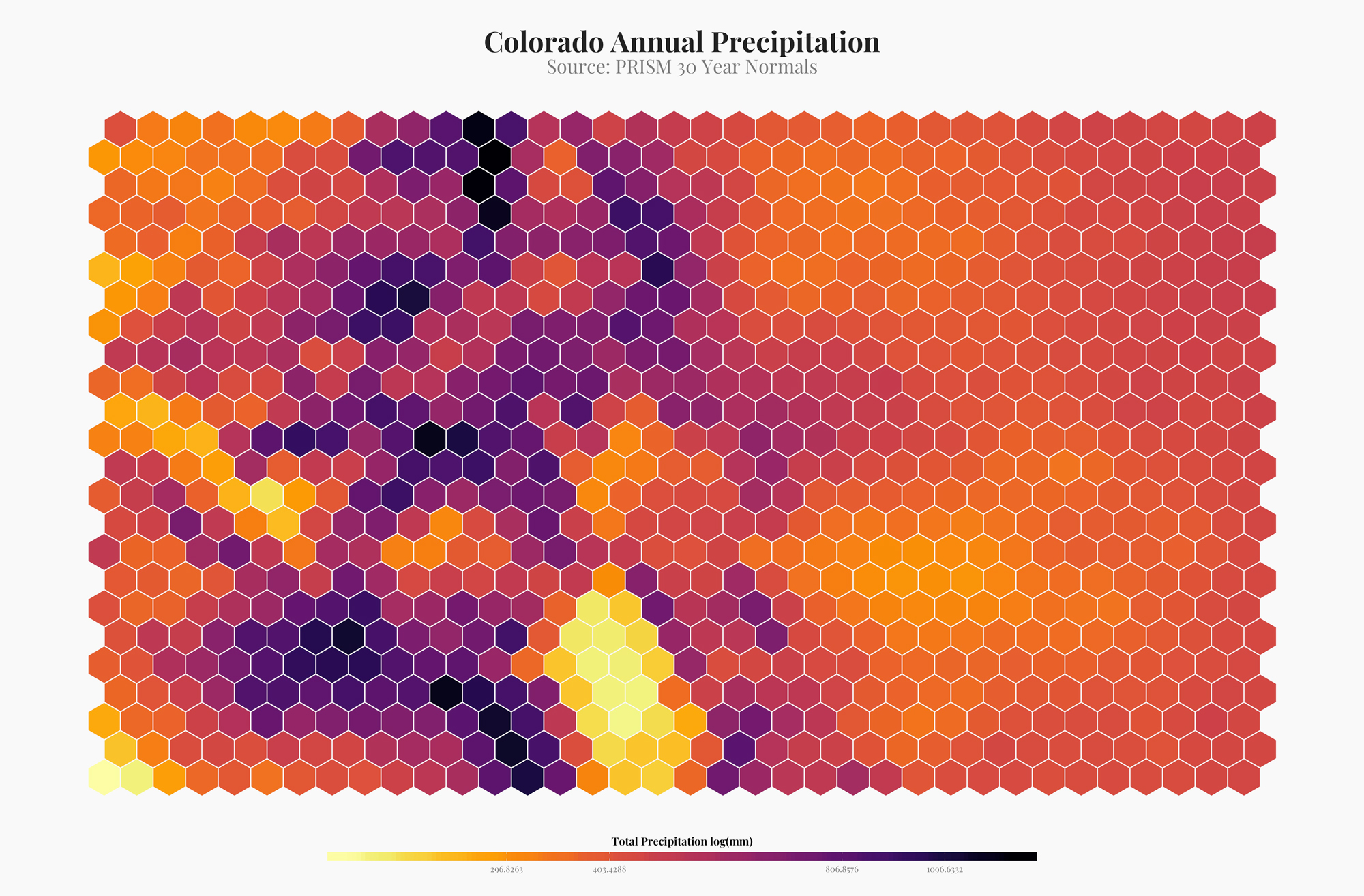
I wanted to look at total annual precipitation throughout the year. We downloaded 30 year normals for each month. Now we just need to add those together and update the raster.
total<-data_cropped_state%>%
  as.data.frame()%>%
  rowSums()

data_cropped_state$total<-total
Now we just need to use the raster with the now calculated totals and extract that data to our state_grid hex grid. We then need to bind the extracted data to the grid and we will be ready to plot.
precip_extract<-extract(x = data_cropped_state,
                       y = as(state_grid, Class = "Spatial"),
                       fun = mean )

precip_hex<-state_grid%>%
  cbind(as_tibble(precip_extract))
The only thing left to do is plot the resulting data using geom_sf with ggplot.
legend_ticks<-c(225, 325, 450, 700, 1050)
precip_hex%>%
  ggplot()+
  geom_sf(aes(fill = total), color = "#f9f9f9")+
  scale_fill_viridis(option = "inferno", direction = -1, trans = "log", breaks = legend_ticks, labels = legend_ticks)+
  labs(title = "Colorado Annual Precipitation",
       subtitle = "Source: PRISM 30 Year Normals",
       fill = "Total Precipitation log(mm)")+
  guides(fill = guide_colourbar(title.position="top", title.hjust = 0.5))+
  ggsave("output/precipitation.jpg", height = 8, width = 11, dpi = 300, units = "in")

?ggsave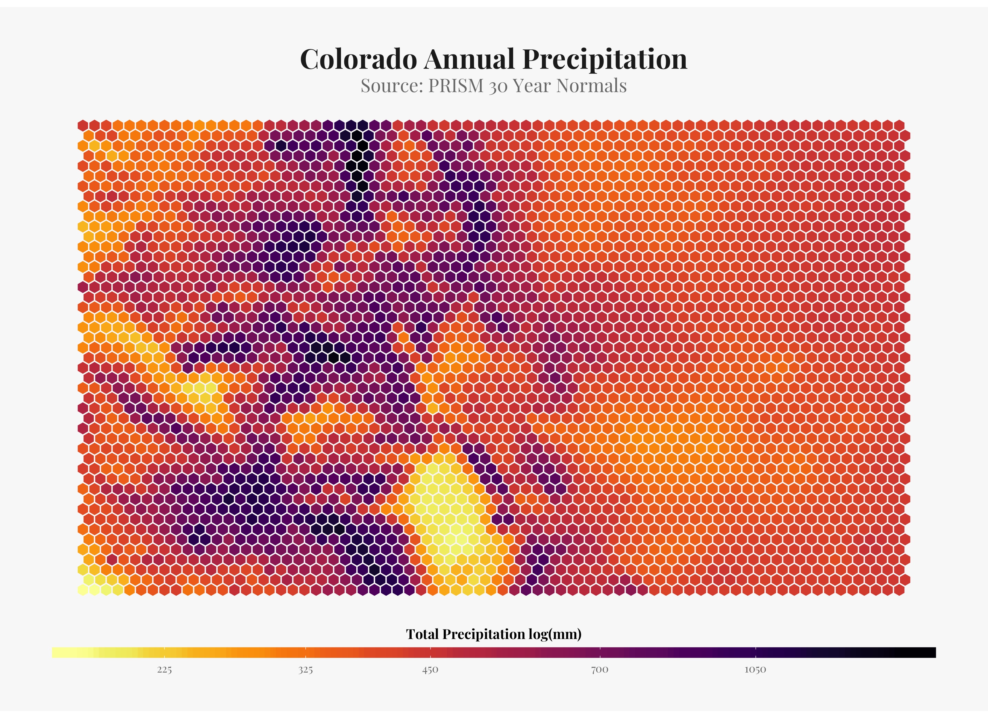
For the rest of these plots, I will just be exploring the data APIs and not go into the process of plotting a hex grid.
Elevation
Download the raster for the state of colorado using the elevatr package and crop it to colorado.
state_dem<-get_elev_raster(as(state_grid, "Spatial"), z = 7)%>%
  crop(state_shape)
Extract the elevation data to the grid we drew before and plot as hex.
dem_extract<-extract(x = state_dem,
                    y = as(state_grid, Class = "Spatial"),
                    fun = mean,
                    na.rm = T)

dem_hex<-state_grid%>%
  cbind(as_tibble(dem_extract))

names(dem_hex)<-c("geometry","dem")

dem_hex%>%
  ggplot()+
  geom_sf(aes(fill = dem), color = "white")+
  scale_fill_viridis(option = "inferno", direction = -1)+
  labs(title = "Colorado Elevation",
       subtitle = "Source: USGS",
       fill = "Elevation (m)")+
  guides(fill = guide_colourbar(title.position="top", title.hjust = 0.5))+
  ggsave("output/elevation.jpg", height = 8, width = 11, dpi = 300, units = "in")
Population
Downlaod the data using the tidycensus package. You can get your census api key here.
options(tigris_use_cache = TRUE) ## because we are going to use block level data a few times we want to cache this shapefile even though it is pretty small.
census_api_key(Sys.getenv("CENSUS_API_KEY")) ## add your own API key here.

v17 <- load_variables(2017, "acs5", cache = TRUE)
View(v17%>%
       dplyr::select(concept, label, name)) ## Look at the avaiable data.

population<-get_acs(geography = "block group",
        variables = c(population ="B01003_001"),
        state = "CO",
        geometry = TRUE) ## Adding geometry true binds the data to a sf object accessed using the tigris package.


pop_final<-population%>%
  mutate(area = as.numeric(st_area(.)), population_by_area = estimate/area)
pop_final%>%
  ggplot()+
  geom_sf(aes(fill = population_by_area), lwd = 0)+
  scale_fill_viridis(option = "inferno", direction = 1, trans = "log")+
  labs(title = "Colorado Population",
       subtitle = "Source: US Census using the tidycensus package",
       fill = "Population log(m^2)")+
  guides(fill = guide_colourbar(title.position="top", title.hjust = 0.5))+
  ggsave("output/population_non_hex.jpg", height = 8, width = 11, dpi = 300, units = "in")

pop_raster<-rasterize(as(pop_final, "Spatial"), data, field = "population_by_area", fun= mean, progress = "text") ## to add the data to the shapefile we first need to rasterize it.


pop_extract<-extract(x = pop_raster,
                    y = as(state_grid, Class = "Spatial"),
                    fun = mean,
                    na.rm = T)


pop_hex<-state_grid%>%
  cbind(as_tibble(pop_extract))%>%
  rename(pop_per_area = V1)

pop_hex%>%
  ggplot()+
  geom_sf(aes(fill = pop_per_area), color = "white")+
  scale_fill_viridis(option = "inferno", direction = -1, trans = "log")+
  labs(title = "Colorado Population",
       subtitle = "Source: US Census using the tidycensus package",
       fill = "Population log(m^2)")+
  guides(fill = guide_colourbar(title.position="top", title.hjust = 0.5))+
  ggsave("output/population.jpg", height = 8, width = 11, dpi = 300, units = "in")
Income
Now we will look at income using the exact same process as above.
income<-get_acs(geography = "block group",
        variables = c(income ="B19013_001"),
        state = "CO",
        geometry = TRUE)

income_final<-income%>%
  mutate(area = as.numeric(st_area(.)), income_by_area = estimate/area)

income_final%>%
  ggplot()+
  geom_sf(aes(fill = estimate), lwd = 0)+
  scale_fill_viridis(option = "inferno", direction = 1, trans = "log")+
  labs(title = "Colorado Income",
       subtitle = "Source: US Census using the tidycensus package",
       fill = "Income log()")+
  guides(fill = guide_colourbar(title.position="top", title.hjust = 0.5))+
  ggsave("output/income_non_hex.jpg", height = 8, width = 11, dpi = 300, units = "in")

income_raster<-rasterize(as(income_final, "Spatial"), data, field = "estimate", fun= mean, progress = "text")


income_extract<-extract(x = income_raster,
                    y = as(state_grid, Class = "Spatial"),
                    fun = mean,
                    na.rm = T)


income_hex<-state_grid%>%
  cbind(as_tibble(pop_extract))%>%
  rename(income = V1)

income_hex%>%
  ggplot()+
  geom_sf(aes(fill = income), color = "#FFFFFF")+
  scale_fill_viridis(option = "inferno", direction = -1, trans = "log")+
  labs(title = "Colorado Income",
       subtitle = "Source: US Census using the tidycensus package",
       fill = "Income log()")+
  guides(fill = guide_colourbar(title.position="top", title.hjust = 0.5))+
  ggsave("output/income.jpg", height = 8, width = 11, dpi = 300, units = "in")