Working with DIMA Tools and Making a Plant List from Species Richness Table
This is a series of notes that works with the DIMA database. The DIMA was produced by the Jornada Research Center for the Assessment Inventory and Monitoring framework.
This R file determines species richness and parses all plants found to make a complete plant list with the number of times they have occurred.
Some useful techniques that are used in it are:
- parsing strings in a column so that each parsed entity is a new entry in a column.
- counting the number of occurrences of a given value within a column.
Load libraries
you must have devtools installed to get dima.tools from here.
##Load Libraries - May need to intall these with install.packages() before loading.
library(RODBC) ## - for reading Access Databases
library(tidyverse)
library(dima.tools)
library(data.table)
library(stringr)
library(ggthemes)
Load the DIMA database.
You can either use read.dima, as I do here. Or you can use the RODBC package like so odbcDriverConnect("Driver={Microsoft Access Driver (*.mdb, *.accdb)};DBQ=database/8_30.mdb"). Note that you must be using 32 bit version of R to connect to an Access Database (either method). to change your r version, go to Tools>Global Options and under the General tab, select change under the "R version" section.
dima<-read.dima("database", all.tables = T)find the species richness table.
species_rich_details<-dima$tblSpecRichDetail
species_rich_details
Subset the species list
We have a lot of blank rows, to eliminate those I added the filter() function to eliminate all of the rows with no plants. Separate rows is used to parse through all of the plant codes.
all_species<-species_rich_details %>%
  filter(SpeciesCount>0)%>%
  select(SpeciesList)%>%
  separate_rows(SpeciesList, convert=T)

View(all_species)
The above code subsets that data and turns this:
| ID | Richness | SpeciesList |
|---|---|---|
| 1 | 3 | ACHY; POFE; BOGR2; |
| 2 | 2 | PLJA; HECO26; |
| 3 | 4 | PIED; ARTR2; DEPI; HECO26 |
Into this:
| ID | SpeciesList |
|---|---|
| 1 | ACHY |
| 2 | POFE |
| 3 | BOGR |
| 4 | PLJA |
| 5 | HECO26 |
| 6 | PIED |
| 7 | ARTR2 |
| 8 | DEPI |
| 9 | HECO26 |
Count each occurrent with table()
This counts each occurrence of each plant and displays it in a table;
count<-as.data.frame(table(all_species$SpeciesList))
final_list<-count%>%
  rename(symbol=1, count=2)
final_list<-final_list[-1, ]
final_list
Load and Merge with the plant list for Colorado
Read the Plant List.
I got this plant list at the USDA Plants Database.
plant_list<-read_csv("COplants5312018.txt")
plant_list
Clean and Merge
The plant list sometimes has more than one entry for each plant. For example ACHY has 3 entries. When you merge it will match all three of those entries, but we only want one of the entries, so we select just the first of each plant instance with match(unique()).
plant_list_cl<- plant_list%>%
  rename(symbol=1, sci_name=3)
plant_list_cl<-plant_list_cl[match(unique(plant_list_cl$symbol), plant_list_cl$symbol),]
plant_list_cl
Join the tables
final_merged_list<-final_list %>%
  left_join(plant_list_cl)%>%
  rename(num_occur=count, common_name=5)%>%
  select(-3)
final_merged_list
Output
The final output should look something like this:
| symbol | count | sci_name | common_name | Family |
|---|---|---|---|---|
| ABCO | 1 | Abies concolor (Gord. & Glend.) Lindl. ex Hildebr. | white fir | Pinaceae |
| ACHY | 24 | Achnatherum hymenoides (Roem. & Schult.) Barkworth | Indian ricegrass | Poaceae |
| ACMI2 | 8 | Achillea millefolium L. | common yarrow | Asteraceae |
| ACRE3 | 1 | Acroptilon repens (L.) DC. | hardheads | Asteraceae |
| ... | ... | ... | ... |
Write the File
write_csv(final_merged_list, "output/species_richness_plant_list_8312018.csv")
Plot
get rid of unknowns
for_plot_cl<-final_merged_list%>%
filter(!str_detect(symbol, "AF"), !str_detect(symbol,"AG01"), !str_detect(symbol,"PF"), !str_detect(symbol, "PG"), !str_detect(symbol, "SH"), !str_detect(symbol,"SU"))%>%
arrange(desc(symbol))
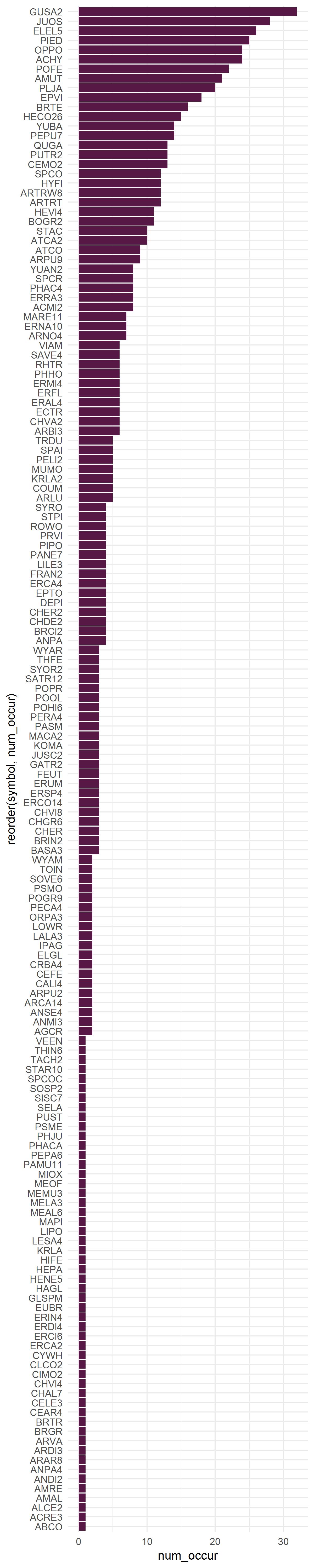
for_plot_clPlot the result and save a copy.
ggplot(for_plot_cl, aes(reorder(symbol, num_occur), num_occur))+
  coord_flip()+
  theme_minimal()+
  geom_col(fill = "#581845")

ggsave("output/frequency_by_symbol.jpg", width = 4, height = 20, units = "in")
The final Result