Making a Chloropleth Map in R
Load the libraries.
library(tidyverse)Load the data and subset the area csv to just the columns we need.
data<-read_csv("https://raw.githubusercontent.com/rfordatascience/tidytuesday/master/data/2018-04-30/week5_acs2015_county_data.csv")
area<-read_csv("/Users/michaelschmidt/Downloads/county_area.csv")%>%
  rename(fips=STCOU, area=LND010190D)%>%
  mutate(CensusId=as.integer(fips))%>%
  select(CensusId,area)
Clean the two datasets and merge them together.
data_cl<-data%>%
  mutate(subregion=tolower(County))%>%
  select(CensusId, subregion, TotalPop)%>%
  left_join(area)%>%
  mutate(people_per_sq_mile=TotalPop/area)%>%
  select(subregion, people_per_sq_mile)
data_cl
Merge the dataset to county data from the maps package.
county<-map_data("county")%>%
  left_join(data_cl)
Plot the data with ggplot using geom_polygon.
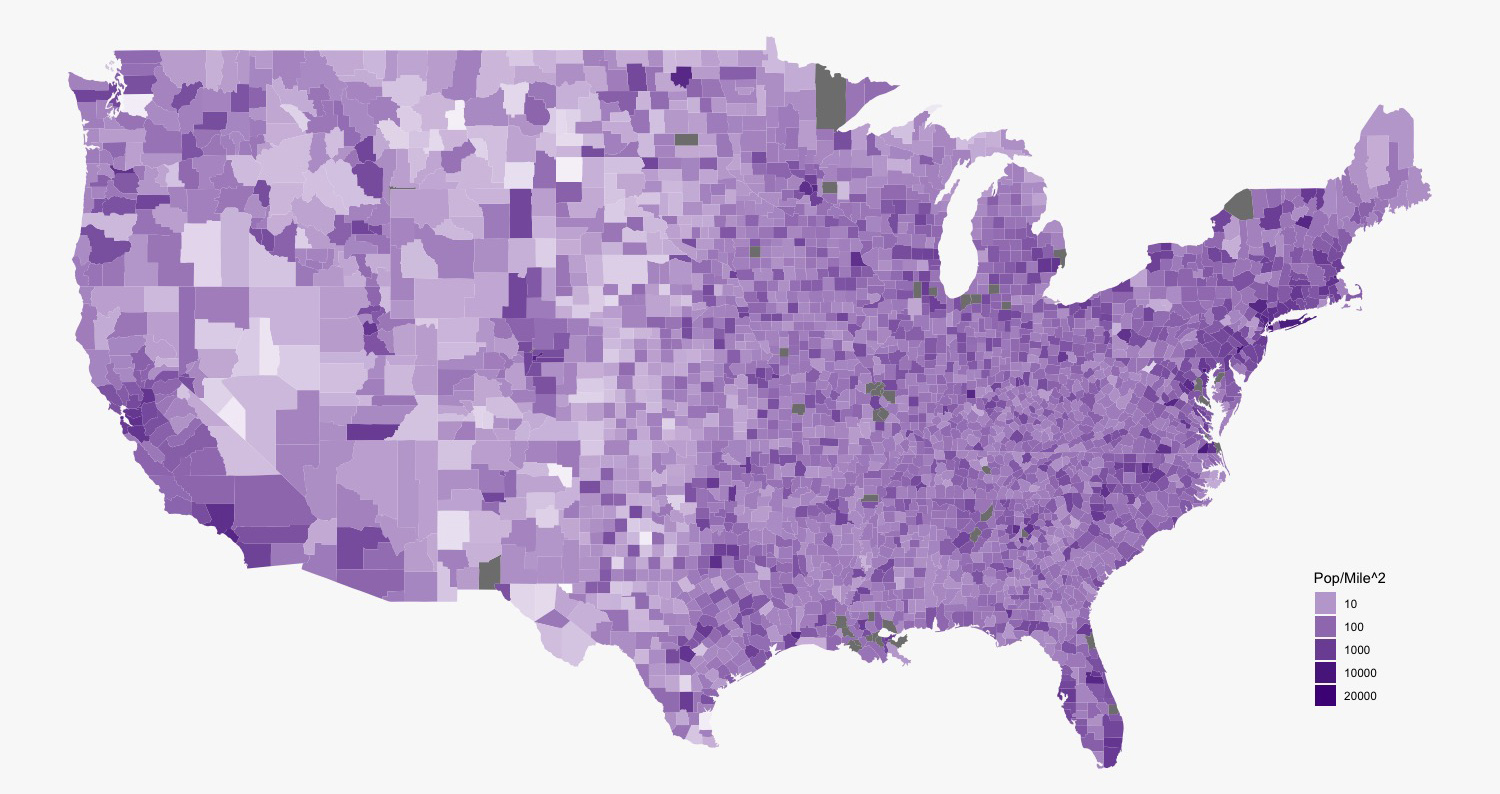
my_breaks <- c(10, 100, 1000, 10000, 20000)
ggplot(data=county)+
  geom_polygon(aes(x=long, y=lat, fill=people_per_sq_mile, group=group))+
  coord_map()+
  scale_fill_gradient(low = "#fcfbfd", high = "#3f007d", trans = "log", breaks = my_breaks, labels = my_breaks)+
  theme_void()+
  guides(fill=guide_legend(title="Pop/Mile^2"))+
  theme(plot.title = element_text(size = 25, face = "bold", hjust = 0.5), panel.background = element_rect(fill = "#f9f9f9"), plot.background = element_rect(fill = "#f9f9f9"), legend.position = c(0.9, 0.2))