Classifying High Resolution Aerial Imagery - Part 1

The following note documents a proof of concept for classifying vegetation with 4 band 0.1m aerial imagery. We used sagebrush, bare ground, grass, and PJ for classes. approximately 300 training polygons were used as a training data.

What I Learned

Success

Random forests was quite successful in classification. The largest error occurred in sagebrush, with an out of bag error of about 3%. However, because this was a first attempt, I did not use a train and validation set. Future iterations of this process should definitely use a more rigorous validation methodology to inform model decisions.

Failures

Shadows presented the biggest challenge to classification. There are two ways to handle this:

• Segmentation - We could try to segment out the shadows prior to classification, and use the shadows as a separate class. We would need to thing about if this would through off any cover estimates. At first thought I would say no, because it would be standardized across a tile.
• Adding in predictors - I think if we used our vegetation polygons as a predictive layer random forests may be able to split the shadows. This would also require us however to draw the shadows as part of a plant so that random forests associates the shadow with the plant/tree.Segementation Resource

Compute power

Compute power was a huge limitation. One tile of imagery is about 12 GB in memory. That's about 1/3 of my 32 GB of memory. I've heard that tensorflow, which uses the GPU, can perform random forests, but I haven't figured out a way to do that in r.

Future Loops

I do not think we have the compute power to perform this process across the entire basin. However, I do think that we could loop through each tile with something like lapply. The next step would be to clean everything up and put the process into a function that you could then predict each tile individually. I think we may need to normalize the statistics on the rasters first however.

Some Results

The Final prediction

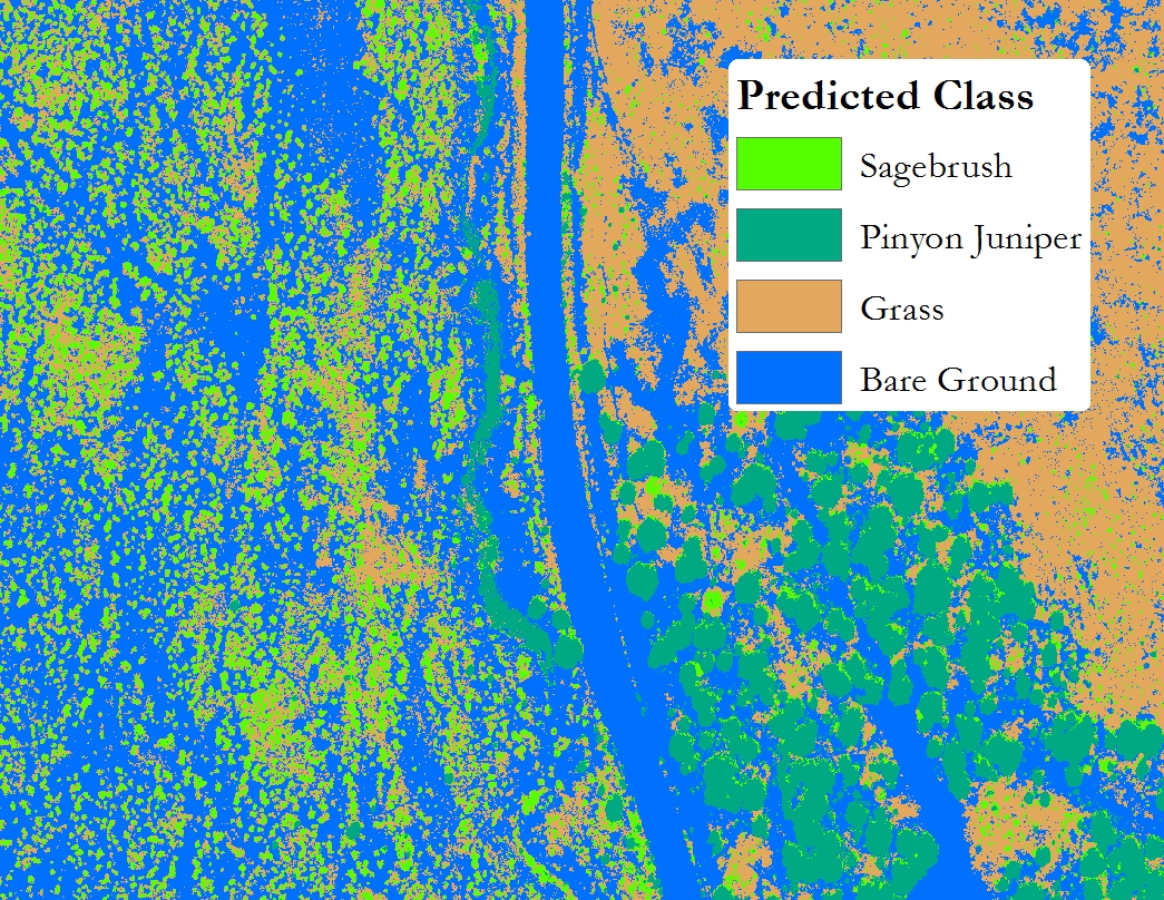
You can see the model did pretty well in classifying the image. However, the failure to classify the PJ shadows correctly is very evident. {: .caption}

The Original Four Band Image

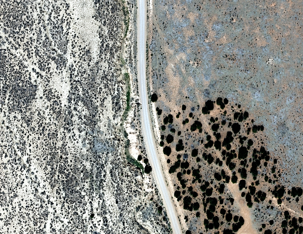
The same extent as the classification raster above. {: .caption}

An example of the training polygons

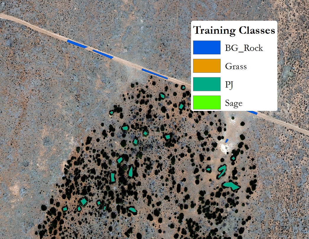
An example of my training polygons. {: .caption}

Notes

If we wanted to publish we would need to validate 50 points per predicted class to statistically validate the process.

R Scripts

Load Libraries

library(raster)
library(tidyverse)
library(randomForest)
library(rgdal)

Load the needed datasets

raster<-brick("data/raster/Basin0301.tif") ## Tile to be classified.
## supervisor<-raster("data/raster/supervisor12N") ## didn't end up using this layer because rasters on a 0.1m scale in ArcMap can't be merged in r because of the decimal error. This applies to test raster as well.
testshape<-readOGR("data/shape", layer="test") ## A subset of Basin0301.tif so that we didn't have to run the prediction on the whole raster.
shape<-readOGR(dsn="data/shape", layer="supervised12N") ## Read in the classification polygons
##test_raster<-raster("data/raster/test_fit") ## I don't remember why I loaded this????

Set up raster and add NDVI layer

names(raster)<-c("b1", "b2", "b3", "b4") ## Rename Bands for ease of use
ndvi<-overlay(raster$b4, raster$b3, fun=function(x,y){(x-y)/(x+y)}) ## Create a NDVI layer
cov<-addLayer(raster,ndvi) ## Merge NDVI and the tiel imagery
names(cov)<-c("b1", "b2", "b3", "b4", "ndvi") ## Rename NDVI to "ndvi", all other layers stay the samel.

Check Alignment

Make sure that the aerial tile has the same extent as the training shapefile using ndvi layer.

plot(ndvi)
plot(shape, add=T)

Convert the Class field to number

shape@data$code<-as.numeric(shape@data$Class)
shape@data

Rasterize the training shapefile

classes<-rasterize(shape, ndvi, field="code")
plot(classes)

Clip and mask

First clip that aerial image to the extent of the classes layer (not the same as ArcMap Clip). Then mask (use classes geometry).

covmask<-crop(cov, extent(classes))
covmask2<-mask(covmask, classes)
plot(covmask2)

Merge Training Dataset to Clipped Dataset.

names(classes)<-"class"
train_brick<-addLayer(covmask2, classes)

Get Values From Raster

I will need to run this step through again to make sure it is correct. For some reason when the aerial raster is clipped to the geometry of the training polygons, all of the clipped out cells remain as NAs (as far as I konw there is no way around this). To run random forests you need to remove the NAs. Removing the NAs took up almost all of my computers memory. I eventually got it to work, by removing everything in memory and then running the filter(train_table2, !is.na(class)) I believe, but I can't quite remember. To do this, I may have needed to save the train_table as a RDS and then re-load it after restarting R so that the machines memory was clean. I'll update once I run this part again, it just takes so long (45min to an hour) I didn't have time to run it twice.

train_table<-getValues(train_brick) ## Takes a lot of time
saveRDS(train_table, "data/train_table2.rds")
train_table<-readRDS("data/train_table2.rds")
library(rgr)
train_table2<-remove.na(train_table)
train_table2<-as.tibble(train_table)
train_table3<-filter(train_table2, !is.na(class))
train_table3

Run Random Forests

Build the model.

set.seed(415)
fit<-randomForest(as.factor(class)~.,
                  data=train_table3,
                  importance=TRUE,
                  ntree=200
                  )
fit ## See the results.
varImpPlot(fit) ## View the most important perdictors.
saveRDS(fit, "data/forests/fit1.rds") ## Save the prediction

Prepare raster datasets to Run the Prediction

Format the datasets into so that the training dataset and the predicted dataset have the same layers (4 light bands and ndvi).

testshape_raster<-rasterize(testshape, raster) ##convert testshape (subset of aerial imagery) to raster with same pixel size as raster.
test_fit<-crop(raster, extent(testshape)) ##crop raster to testshape
plot(test_fit) ##Look at test fit
names(test_fit)<-c("b1", "b2", "b3", "b4") ## rename testfit names to match training set.
ndvi2<-overlay(test_fit$b4, test_fit$b3, fun=function(x,y){(x-y)/(x+y)}) ## add ndvi
test_fit_comb<-addLayer(test_fit, ndvi2) ## Merge the layers
names(test_fit_comb)<-c("b1", "b2", "b3", "b4", "ndvi") ##rename ndvi header to ndvi.

Run the prediction on the data subest and the whole dataset.

predicted_plot<-raster::predict(test_fit_comb, fit, OOB=T) ## Predict subset
##predicted_whole<-raster::predict(cov, fit, OOB=T) ## predict whole dataset - This takes over an hour with a 32GB machine.

Save everything

When you write the rasters with writeRaster the rasters still need to be projected once they are pulled into ArcMap. I'm srue there is a way to save them with a projection, but I haven't figured it out yet.

saveRDS(predicted_plot, "data/forests/predicted_raster.rds")
saveRDS(predicted_whole, "data/forests/predicted_whole_raster.rds")
predicted_plot2<-predicted_plot

writeRaster(predicted_plot2, "data/raster/prediction.asc")
writeRaster(predicted_whole, "data/raster/prediction_whole.asc")