Predicting if the Dolores River Will Have a Raftable Release V2
Will there be a raftable release below McPhee Dam this year? I hope so. In this post I'll use the {tidymodels} R package to predict the number of raftable release days with Xgboost. This post is an update to an earlier post. I take a slightly different approach to build this model and I think the model is more accurate than the last model I built.
Update: I put up an updated model prediction to this here. It improves drastically on the model below. I basically changed the engine to xgboost count/poisson instead of regular regression because raftable release days is essentially count data. To do this when setting the engine for the parsnip model you just add a option parameter: `set_engine("xgboost", option="count:poisson").
All the packages I will be using
First lets load all the packages we will need to get the data.
library(snotelr)
library(tidyverse)
library(lubridate)
library(RNRCS)
library(pscl)
library(tidymodels)
library(poissonreg)
library(MetBrewer)
library(extrafont)
loadfonts()

theme_set(theme_minimal(base_family="Inter Medium"))
theme_update(
  plot.title=element_text(family="Inter ExtraBold"),
  legend.position=c(0.8,0.1),
  legend.direction="horizontal"
)
Getting the data
We need three datasets to make the prediction:
- Snow pack data - we get this from the NRCS SNOTEL network using the
{snotelr}. We will get water equivalent data for four sites: El Diente Peak, Lizard Head Pass, and Lone Cone and Scotch Creek. These sites were selected because they go back to when the damn was built and they cover a few different areas within the Dolores River Drainage. Admittedly I wish they were a bit more spread out. - McPhee Dam Volume - two things go into if the McPhee will fill up and have enough excess to have a spill at a raftable level: the current damn volume and the current snowpack. To get the McPhee dam daily volume I used the
{RNRCS}package. In the past I used this package to get the SNOTEL site data as well but for some reason I couldn't get it to work this go round. - River Flow Rates Below McPhee Dam - To determine if a raftable release has occurred you need to know what the river level is below McPhee Dam. For this we pull data from the USGS Stream Flow Gauge at Bedrock, Colorado. For this I just used the USGS Water Services API which can produce a TSV.
Pull the Snow Water Equivalent Data Using {snotelr}
We need daily snow water equivalent data for the four sites: El Diente Peak, Lizard Head Pass, and Lone Cone and Scotch Creek. To be clear, I used these sites because I used them in my last analysis. It might be good to review if there are any better sites to use. I remember picking these because I thought it would be good to have sites at different elevations above McPhee so that I could capture some elevational nuance in the snowpack. But these sites are all pretty high. To get the snowpack data we use a function that uses the elevatr::snotel_download() function that takes a site_id as an argument. We can use this function which I've called get_snotel_data to loop over each site id and return a tibble of daily snotel numbers.
dolores_site_ids<-c(465, 586, 589, 739)

get_snotel_data<-function(site_id){
  snotel_download(site_id = site_id, internal=TRUE)%>%
    as_tibble()
}

all_sntl_data<-lapply(dolores_site_ids, get_snotel_data)%>%
  bind_rows()

sntl_cl<-all_sntl_data%>%
  select(site_id, date, snow_water_equivalent)%>%
  mutate(date=as.Date(date))
At the end we select just the variables we need and convert the date to an actual date. The resulting dataframe looks something like this.
>snotel_cl
# A tibble: 57,693 × 3
   site_id date       snow_water_equivalent
     <dbl> <date>                     <int>
 1     465 1986-08-05                    NA
 2     465 1986-08-06                     0
 3     465 1986-08-07                     0
 4     465 1986-08-08                     0
 5     465 1986-08-09                     0
 6     465 1986-08-10                     0
 7     465 1986-08-11                     0
 8     465 1986-08-12                     0
 9     465 1986-08-13                     0
10     465 1986-08-14                     0
# … with 57,683 more rows
# ℹ Use `print(n = ...)` to see more rows
The last steps are to get just the years after McPhee was put in, convert the site ids to better header formats and then pivot the data so that each date has a value for each of the four sites.
all_sites_sntl<-sntl_cl%>%
  filter(year(date)>1986)%>%
  mutate(site_id = paste0("site_id_", site_id))%>%
  pivot_wider(names_from=site_id, values_from=snow_water_equivalent)
> all_sites_sntl
# A tibble: 13,172 × 5
date site_id_465 site_id_586 site_id_589 site_id_739
<date> <int> <int> <int> <int>
1 1987-01-01 122 175 124 99
2 1987-01-02 124 183 130 102
3 1987-01-03 124 185 132 102
4 1987-01-04 124 183 137 104
5 1987-01-05 130 183 137 107
6 1987-01-06 145 196 168 112
7 1987-01-07 145 196 173 112
8 1987-01-08 155 188 185 112
9 1987-01-09 155 180 190 124
10 1987-01-10 155 175 193 124
# … with 13,162 more rows
# ℹ Use `print(n = ...)` to see more rowsWe now have the data for four snotel sites that we will be joining with the rest of the datasets.
Pulling Reservoir Volume Using {RNRCS}
The Bureau of Reclemation (BOR, the agency that manages McPhee Dam) is a bit easier. The {RNRCS} package has a nifty function grabBOR.data() that takes: site_id, timescale, Daybgn, and DayEnd. After a little cleaning we have a joinable dataset to the snotel data above.
bor_data<-grabBOR.data(site_id = "MPHC2000",
                       timescale = 'daily',
                       DayBgn = "1987-01-01",
                       DayEnd = Sys.Date())%>%
  as_tibble()%>%
  mutate(date = as.Date(Date),
         res_volume = as.numeric(`Reservoir Storage Volume (ac_ft) Start of Day Values`))%>%
  select(date, res_volume)
> bor_data
r$> bor_data
# A tibble: 13,172 × 2
date res_volume
<date> <dbl>
1 1987-01-01 293384
2 1987-01-02 293423
3 1987-01-03 293460
4 1987-01-04 293535
5 1987-01-05 293610
6 1987-01-06 293574
7 1987-01-07 293574
8 1987-01-08 293610
9 1987-01-09 293649
10 1987-01-10 293610
# … with 13,162 more rows
# ℹ Use `print(n = ...)` to see more rowsAt the onset, it doesn't seem probable that a raftable release will occur. To have a raftable release, we need McPhee reservoir to fill up, having excess water to spill below the damn. Looking at all volumes for January 1st, this year is the eighth lowest reservoir volume since 1987 (as far back as I have data for).
bor_data%>%
  filter(month(date)=="1" & day(date)=="1")%>%
  arrange(res_volume)
# A tibble: 37 × 2
   date       res_volume
   <date>          <dbl>
 1 2003-01-01     159438
 2 2022-01-01     164790
 3 2021-01-01     167774
 4 2019-01-01     168033
 5 2004-01-01     171742
 6 2015-01-01     181336
 7 2014-01-01     182394
 8 2023-01-01     186844
 9 2013-01-01     192216
10 2005-01-01     205100
# … with 27 more rows
# ℹ Use `print(n = ...)` to see more rows
But after a ton of snow in January I thought that maybe we could have a release.
Now we join these datasets to get all of our predictors or variables....almost. We need to make one more variable to keep track of the season which we will take care of in a later step.
vars_all<-all_sites_sntl%>%
  left_join(bor_data, by="date")
> vars_all
# A tibble: 13,172 × 6
date site_id_465 site_id_586 site_id_589 site_id_739 res_volume
<date> <int> <int> <int> <int> <dbl>
1 1987-01-01 122 175 124 99 293384
2 1987-01-02 124 183 130 102 293423
3 1987-01-03 124 185 132 102 293460
4 1987-01-04 124 183 137 104 293535
5 1987-01-05 130 183 137 107 293610
6 1987-01-06 145 196 168 112 293574
7 1987-01-07 145 196 173 112 293574
8 1987-01-08 155 188 185 112 293610
9 1987-01-09 155 180 190 124 293649
10 1987-01-10 155 175 193 124 293610
# … with 13,162 more rows
# ℹ Use `print(n = ...)` to see more rowsDolores Raftable Release Days Per Year
This one is a bit more involved. We need to pull daily totals for the Bedrock gauge and then by year calculate how many days are above 800 cfs (what I consider the raftable limit).
I'm not going to go over the USGS water services REST API here but it is well documented and you can generate a URL here.
url<-paste0("https://waterservices.usgs.gov/nwis/dv/?format=rdb&sites=09169500,%2009166500&startDT=1985-02-01&endDT=", Sys.Date(), "&statCd=00003&siteType=ST&siteStatus=all")

flow_data<-read_tsv(url, skip = 35)%>%
  select(2:5)%>%
  rename(site_id = 1, date = 2, flow=3, code = 4)%>%
  mutate(
    site_id = ifelse(site_id == "09166500", "Dolores", "Bedrock"),
    flow=as.numeric(flow)
  )%>%
  drop_na()
Just a note, here I get data for both Bedrock and Dolores. I did this originally because I thought that I would be using inflows too. Really though the snow water equivalent will create the inflows so it doesn't matter what the inflows are if you have the snow water equivalent.
Some cleaning and munging give us the number of days of runoff above 800 cfs per year. The steps are:
- filter just the bedrock site.
- create a raftable day field and all days that are raftable get a value of 1. Non-raftable days get a 0.
- create a year field to summarize the data.
- filter months so we just have the dates when runoff occurs and we don't get any noise from flash flood events.
- sum all days that are raftable within a given year.
predicted_variable<-flow_data%>%
  filter(site_id=="Bedrock")%>%
  mutate(
    raftable = ifelse(flow>800, 1, 0),
    year = year(date)
  )%>%
  filter(month(date) %in% c(3:7))%>%
  group_by(year)%>%
  summarize(raftable_release_days = sum(raftable))%>%
  ungroup()
> predicted_variable
# A tibble: 38 × 2
year raftable_release_days
<dbl> <dbl>
1 1985 102
2 1986 85
3 1987 87
4 1988 13
5 1989 17
6 1990 0
7 1991 9
8 1992 61
9 1993 99
10 1994 35
# … with 28 more rows
# ℹ Use `print(n = ...)` to see more rowsWe have two things left to do. Join the predictors and the predicted variable and create an index to runoff. The index to runoff just keeps track of how close you are to runoff in a general way. I somewhat randomly decided that the index would consist of 12 values. The higher the index the closer to runoff you are. I'm hoping that the model will realize that the higher the index the more accurate the model is. I'm stretching here a little bit. I tried to figure out how to add a date to event type predictor but this is as good as I could do.
data_all<-vars_all%>%
  mutate(year=year(date))%>%
  left_join(predicted_variable, by="year")%>%
  mutate(total = site_id_465+site_id_586+site_id_589+site_id_739)%>%
  filter(total!=0)%>%
  select(-total)%>%
  mutate(
    yday = yday(date),
    dummy = yday-170,
    day_to_runoff = if_else(dummy<1, dummy+365, dummy),
    index_to_runoff = round(day_to_runoff/30),
    raftable_release_days = ifelse(is.na(raftable_release_days), 0, raftable_release_days)
  )%>%
  select(-yday, -dummy)
The last thing we do here is remove as many days that are zero for all of the snotel sites. And now we have our dataset ready to build our model.
data_all
# A tibble: 7,598 × 10
date site_id_465 site_id_586 site_…¹ site_…² res_v…³ year rafta…⁴ day_t…⁵ index…⁶
<date> <int> <int> <int> <int> <dbl> <dbl> <dbl> <dbl> <dbl>
1 1987-01-01 122 175 124 99 293384 1987 87 196 7
2 1987-01-02 124 183 130 102 293423 1987 87 197 7
3 1987-01-03 124 185 132 102 293460 1987 87 198 7
4 1987-01-04 124 183 137 104 293535 1987 87 199 7
5 1987-01-05 130 183 137 107 293610 1987 87 200 7
6 1987-01-06 145 196 168 112 293574 1987 87 201 7
7 1987-01-07 145 196 173 112 293574 1987 87 202 7
8 1987-01-08 155 188 185 112 293610 1987 87 203 7
9 1987-01-09 155 180 190 124 293649 1987 87 204 7
10 1987-01-10 155 175 193 124 293610 1987 87 205 7
# … with 7,588 more rows, and abbreviated variable names ¹site_id_589, ²site_id_739,
# ³res_volume, ⁴raftable_release_days, ⁵day_to_runoff, ⁶index_to_runoff
# ℹ Use `print(n = ...)` to see more rowsBuilding a few models.
The last thing we need to do before we make a model is split the data into two. The first dataset will be all dates from this winter (2022/2023) because we will use the model we make to predict on these dates. We don't yet know what the runoff will be this winter so it won't be helpful in building the model. And the other will be the rest of the data from our dataset. So everything but this winter.
data_known<-data_all%>%
  filter(date<"2022-06-01")

this_year<-data_all%>%
  filter(date>"2022-06-01")
Xgboost Tidymodel Prediction
We'll use XGboost to make the model. I also tried Poisson and Zero Inflated models but neither performed close XGboost. I'd also say it is a good idea to do a bit of data exploration prior to this step, which I did, but was a bit much to write about and include in this post.
To build that model, we first set a seed to make our results repeatable. We then split the data into training and testing and set the model specification. The specification in this case lays out the XGboost parameters that we want to tune and that we are performing a regression.
set.seed(1234)
split<-initial_split(data_known, strata=year)
train<-training(split)
test<-testing(split)

## XGboost
xgb_spec<-boost_tree(
  trees=1000,
  tree_depth = tune(),
  min_n = tune(),
  loss_reduction = tune(),
  sample_size = tune(),
  mtry = tune(),
  learn_rate = tune()
)%>%
set_engine("xgboost")%>%
set_mode("regression")

xgb_spec
> xgb_spec
Boosted Tree Model Specification (regression)
Main Arguments:
mtry = tune()
trees = 1000
min_n = tune()
tree_depth = tune()
learn_rate = tune()
loss_reduction = tune()
sample_size = tune()
Computational engine: xgboost Next, we set up a table of parameters to tune the XGboost model. XGboost is easy to overfit. So parameter tuning is important. We make parameter combinations that we would like to tune with grid_latin_hpyercube(). Here we chose to tune all parameters using 30 combinations.
xgb_grid<-grid_latin_hypercube(
  tree_depth(),
  min_n(),
  loss_reduction(),
  sample_size = sample_prop(),
  finalize(mtry(), train),
  learn_rate(),
  size=30
)

xgb_grid
> xgb_grid
# A tibble: 30 × 6
tree_depth min_n loss_reduction sample_size mtry learn_rate
<int> <int> <dbl> <dbl> <int> <dbl>
1 2 15 1.40e- 9 0.845 2 1.15e- 4
2 1 35 2.98e- 3 0.444 2 6.96e- 6
3 11 20 2.15e-10 0.132 3 3.14e- 4
4 6 28 1.56e+ 1 0.592 8 2.56e- 2
5 7 7 2.96e- 6 0.855 8 1.47e- 8
6 5 37 6.63e- 4 0.977 2 6.87e- 2
7 6 36 1.22e- 8 0.781 3 3.78e- 7
8 4 11 1.28e+ 1 0.205 3 2.33e-10
9 9 18 2.28e- 2 0.579 5 7.40e- 8
10 13 24 8.44e- 8 0.713 7 8.14e-10
# … with 20 more rows
# ℹ Use `print(n = ...)` to see more rowsNext we specify a workflow which includes the formula for the model and the model specification which we created above.
xgb_wf<-workflow()%>%
  add_formula(raftable_release_days~site_id_465+site_id_586+site_id_589+site_id_739+res_volume+index_to_runoff)%>%
  add_model(xgb_spec)

xgb_wf
> xgb_wf
══ Workflow ═════════════════════════════════════════════════════════════
Preprocessor: Formula
Model: boost_tree()
── Preprocessor ─────────────────────────────────────────────────────────
raftable_release_days ~ site_id_465 + site_id_586 + site_id_589 +
site_id_739 + res_volume + index_to_runoff
── Model ────────────────────────────────────────────────────────────────
Boosted Tree Model Specification (regression)
Main Arguments:
mtry = tune()
trees = 1000
min_n = tune()
tree_depth = tune()
learn_rate = tune()
loss_reduction = tune()
sample_size = tune()
Computational engine: xgboost Next we further split our data by year to make several pairs to train and then test the data for each parameter combination. Like I said above XGboost can over fit your data so this step helps us determine how generalizable the model will be. It is testing for each fold, does this data work for the part we leave out?
set.seed(2345)

vb_folds<-vfold_cv(train, strata=year)

vb_folds
> vb_folds
# 10-fold cross-validation using stratification
# A tibble: 10 × 2
splits id
<list> <chr>
1 <split [5060/565]> Fold01
2 <split [5062/563]> Fold02
3 <split [5062/563]> Fold03
4 <split [5063/562]> Fold04
5 <split [5063/562]> Fold05
6 <split [5063/562]> Fold06
7 <split [5063/562]> Fold07
8 <split [5063/562]> Fold08
9 <split [5063/562]> Fold09
10 <split [5063/562]> Fold10We then run the tuning. This step takes a while because it is running th model for each parameter set on each fold. We use doParallel here to use multiple cores to speed things up.
library(doParallel)
doParallel::registerDoParallel()

set.seed(3456)

xgb_res<-tune_grid(
  xgb_wf,
  resamples = vb_folds,
  grid = xgb_grid,
  control = control_grid(save_pred = TRUE)
)
> xgb_res
# Tuning results
# 10-fold cross-validation using stratification
# A tibble: 10 × 5
splits id .metrics .notes .predi…¹
<list> <chr> <list> <list> <list>
1 <split [5060/565]> Fold01 <tibble [60 × 10]> <tibble [1 × 3]> <tibble>
2 <split [5062/563]> Fold02 <tibble [60 × 10]> <tibble [1 × 3]> <tibble>
3 <split [5062/563]> Fold03 <tibble [60 × 10]> <tibble [1 × 3]> <tibble>
4 <split [5063/562]> Fold04 <tibble [60 × 10]> <tibble [1 × 3]> <tibble>
5 <split [5063/562]> Fold05 <tibble [60 × 10]> <tibble [1 × 3]> <tibble>
6 <split [5063/562]> Fold06 <tibble [60 × 10]> <tibble [1 × 3]> <tibble>
7 <split [5063/562]> Fold07 <tibble [60 × 10]> <tibble [1 × 3]> <tibble>
8 <split [5063/562]> Fold08 <tibble [60 × 10]> <tibble [1 × 3]> <tibble>
9 <split [5063/562]> Fold09 <tibble [60 × 10]> <tibble [1 × 3]> <tibble>
10 <split [5063/562]> Fold10 <tibble [60 × 10]> <tibble [1 × 3]> <tibble>
# … with abbreviated variable name ¹.predictions
collect_metrics(xgb_res)%>%
filter(.metric=="rmse") %>%
select(mean, mtry:sample_size) %>%
pivot_longer(mtry:sample_size,
values_to = "value",
names_to = "parameter"
) %>%
ggplot(aes(value, mean, color = parameter)) +
geom_point(alpha = 0.8, show.legend = FALSE) +
facet_wrap(~parameter, scales = "free_x") +
scale_color_manual(values = met.brewer("Isfahan1", 6))+
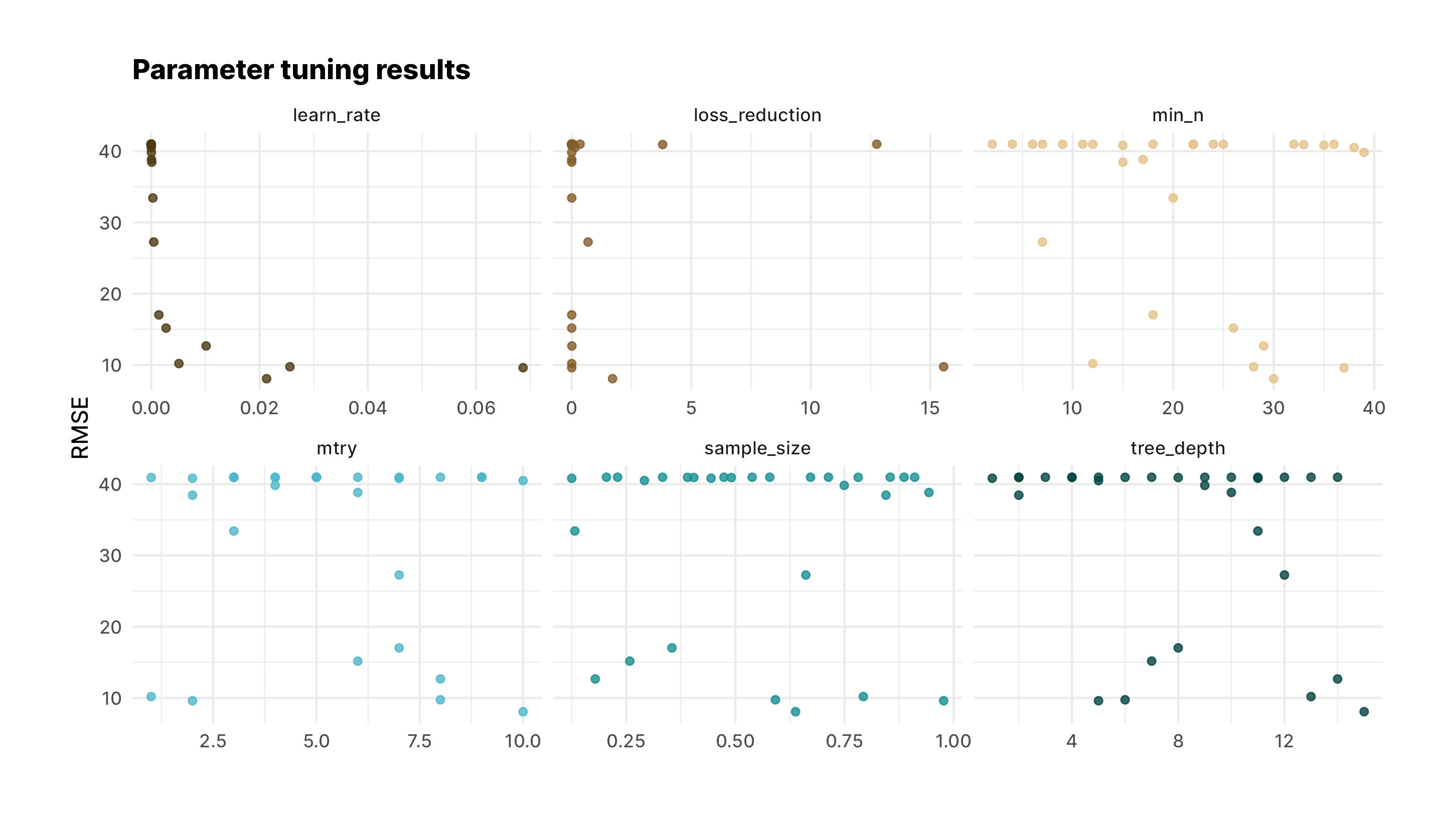
labs(title="Parameter tuning results", x = NULL, y = "RMSE")+
ggsave("output/parameter_tuning_results_xgb.jpg")It looks like there are several parameter sets to choose from. We'll pick one of the best and finalize the workflow.
best_rmse <- select_best(xgb_res, "rmse")

final_xgb <- finalize_workflow(
  xgb_wf,
  best_rmse
)
> final_xgb
══ Workflow ═════════════════════════════════════════════════════════════
Preprocessor: Formula
Model: boost_tree()
── Preprocessor ─────────────────────────────────────────────────────────
raftable_release_days ~ site_id_465 + site_id_586 + site_id_589 +
site_id_739 + res_volume + index_to_runoff
── Model ────────────────────────────────────────────────────────────────
Boosted Tree Model Specification (regression)
Main Arguments:
mtry = 10
trees = 1000
min_n = 30
tree_depth = 15
learn_rate = 0.0213020107597359
loss_reduction = 1.70921120206264
sample_size = 0.637869277962018Next we'll look at feature importance to see what variables were most helpful for the model.
library(vip)

final_xgb %>%
  fit(data = train) %>%
  extract_fit_parsnip() %>%
  vip(geom = "point")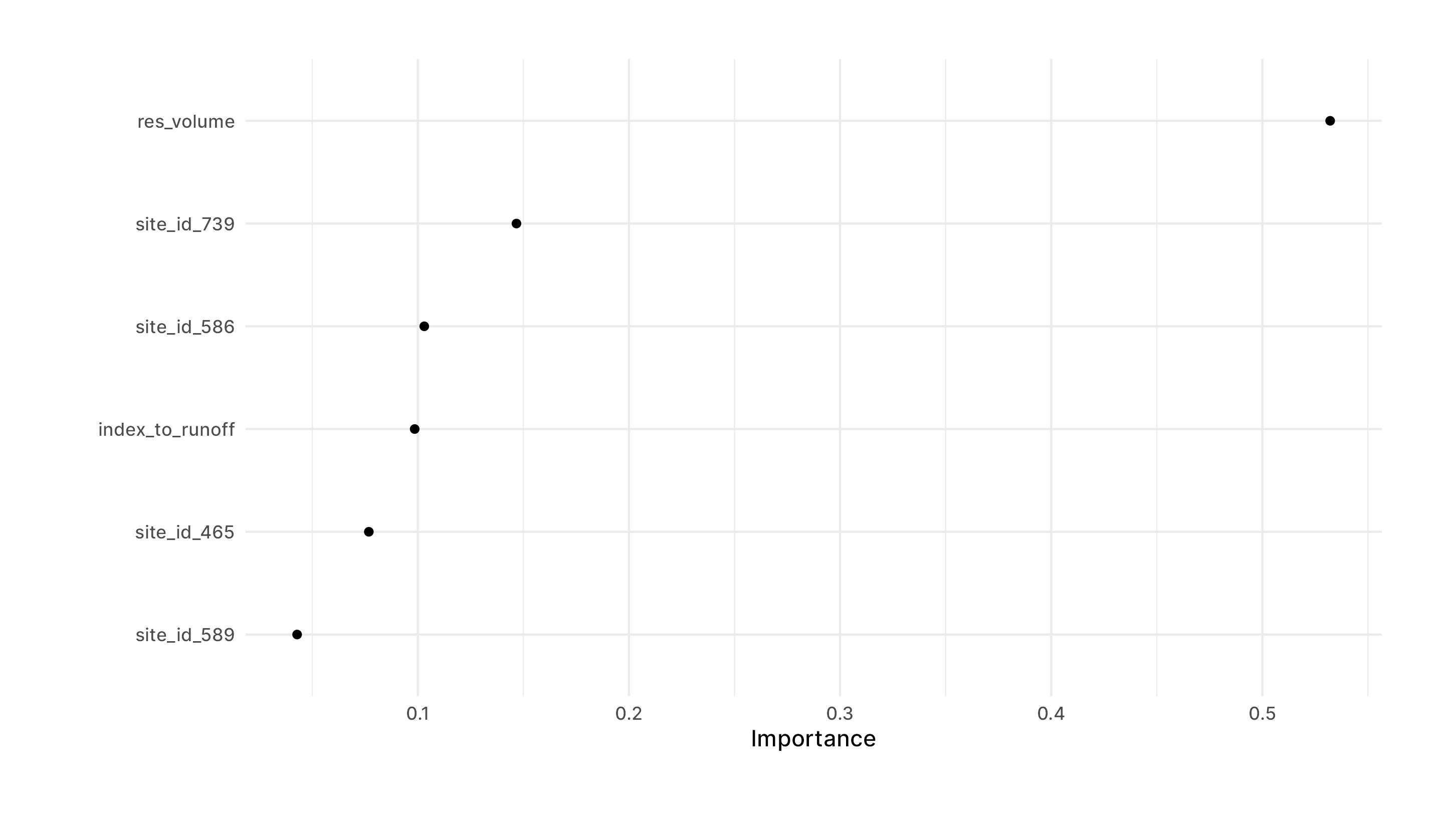
Interestingly Scotch Creek which is one of the lower snotel sites is the most important for the model. That makes sense to me because years when we have lots of low elevation snow are years when we have the best snowpack. Also as expected, reservoir volume is by far the most important, which makes sense.
Note: here we could do some more comparison of the test results to the training results and I'll probably do that in the future. But for now, because I'm running out of time we are just going to make last prediction with best parameters and apply it to all the data. Then let's look at the comparison between the actual release days and the predicted.
final_res <- last_fit(final_xgb, split)

data_all%>%
  bind_cols(predict(extract_workflow(final_res), .))%>%
  ggplot(aes(raftable_release_days, .pred, color = index_to_runoff))+
  geom_point(size=4, alpha=0.3)+
  scale_color_gradientn(
    colors = met.brewer("Isfahan1"),
    guide=guide_colourbar(
      title.position="top",
      barwidth=10,
      barheight=0.5
    )
  )+
  labs(
    title="XGboost Model Dolores River Predict",
    subtitle="Comparison of Actual Days of Raftable Releases to Model Prediction",
    x = "Raftable Release Days Actual",
    y = "Predicted Raftable Release Days",
    color="Time to Runoff Index"
  )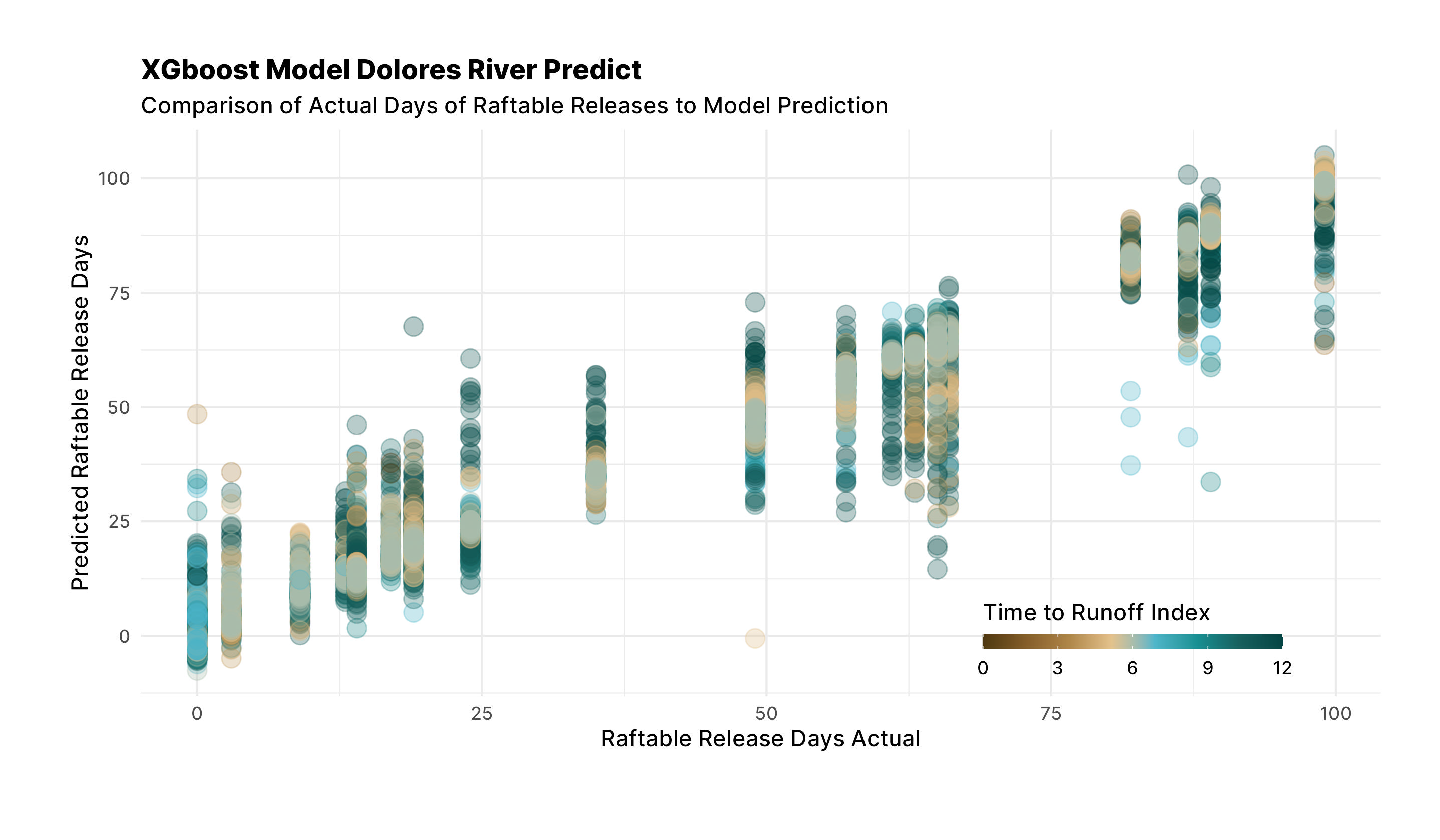
Things look pretty good. Now let's apply the model to this years data and see what we get. Two things jump out at me: the predictions seem to be centering near the actual runoff values and that the model tends to get closer as the index to runoff gets closer to the date for some years. One thing we don't account for in this model, spring rains, and so this model will never be perfect. Let's apply the model to this year.
this_year%>%
  filter(date>as.Date("2022-11-01"))%>%
  bind_cols(predict(extract_workflow(final_res), .))%>%
  ggplot(aes(date, .pred))+
  geom_smooth()+
  geom_point()+
  labs(
    title="Winter 2022/2023 Dolores River Release Prediction",
    subtitle=paste0("Over Time as of ", Sys.Date()),
    x="",
    y="Predicted Number of Days"
  )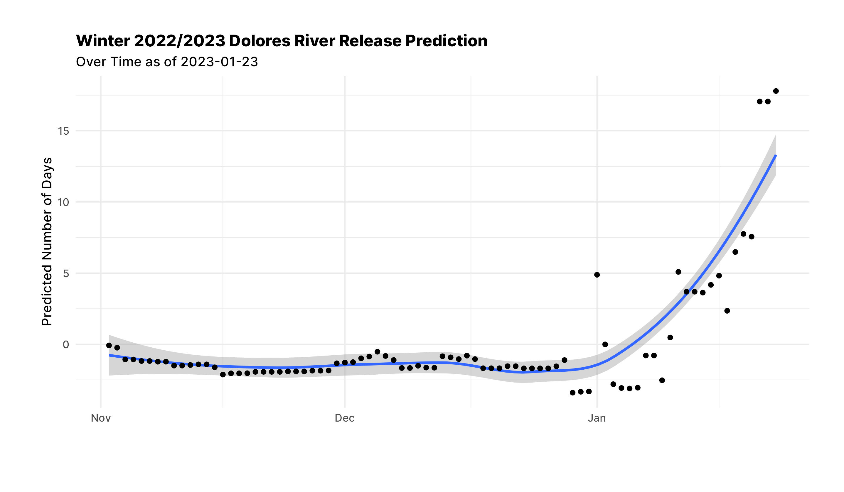
As of this last storm the model is trending towards a 15 day release. We have another storm coming this next week. I'd like to see if the predicted days continue to increase.
I'm also going to try and add this model to a server so that we can always have an up to date prediction. Not totally sure how to do that yet. I might put it up with a new post.