Kernel Density Estimation in R

For a recent project I needed to run a kernel density estimation in R, turning GPS points into a raster of point densities. Below is how I accomplished that.

Load the needed libraries

library(sf)
library(raster)
library(ggspatial)

If you don't have these packages you need to run install.packages(c("sf", "raster")) before they can be loaded.

Create XY Points

For the purposes of this exercise, and because the original dataset I worked with is not available to the public, we will not be loading a shapefile but instead making one out of randomly generated X and Y coordinates. We will create UTM coordinates in Zone 13. You could also create Latitude and Longitude coordinates if you wanted. Here are the bounds of the coordinates:

Northing max: 4232607
Northing min: 4220932

Easting max: 187973
Easting min: 173118

We'll use rnorm to generate 20000 coordinate pairs randomly. You could also use runif but rnorm creates areas with higher densities so our plot is not uniform.

coord<-tibble(
  northing = rnorm(10000, 4220105, 3589.521),
  easting = rnorm(10000, 185310.8, 12709.06)
)

Now we can plot the results to verify the points were generated correctly.

coord%>%
  ggplot(aes(northing, easting))+
    geom_point(color = "steelblue", size = 3, alpha = 0.35)+
    theme_minimal()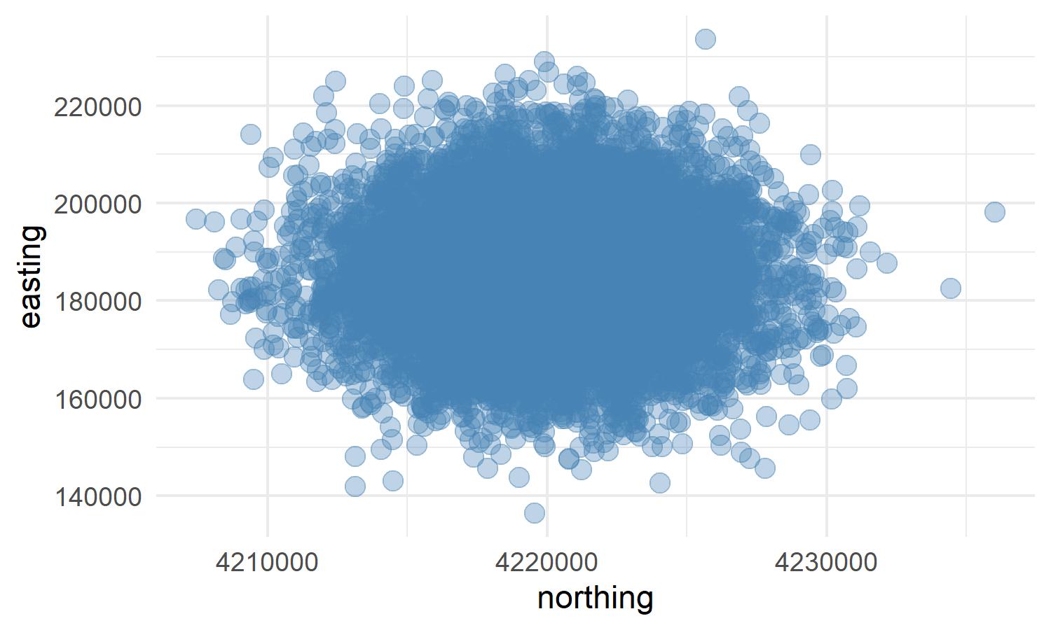

Everything looks good. Now we need to convert the xy coordinates to a shapefile.

Converting xy coordinates to a shapefile

Now that we have xy pairs we can easily convert the xy pairs to a shapefile and give the shapefile a projection. If you need more info on projections you can find it here

sf_obj<- st_as_sf(coord, coords = c("easting", "northing"), crs = "+proj=utm +zone=13 +ellps=GRS80 +datum=NAD83 +units=m +no_defs")

sf_obj

Output:

Simple feature collection with 5000 features and 0 fields
geometry type:  POINT
dimension:      XY
bbox:           xmin: 173118.4 ymin: 4220933 xmax: 187971.9 ymax: 4232603
epsg (SRID):    26913
proj4string:    +proj=utm +zone=13 +ellps=GRS80 +towgs84=0,0,0,0,0,0,0 +units=m +no_defs
# A tibble: 5,000 x 1
             geometry
          <POINT [m]>
 1 (176681.1 4230659)
 2 (174927.8 4222673)
 3 (178167.1 4229261)
 4 (186605.6 4230476)
 5 (176185.4 4227015)
 6 (184934.5 4222134)
 7 (186177.4 4231785)
 8   (183417 4231574)
 9 (187055.3 4222734)
10   (174989 4230511)
# ... with 4,990 more rows

Let's take a look at our new shapefile.

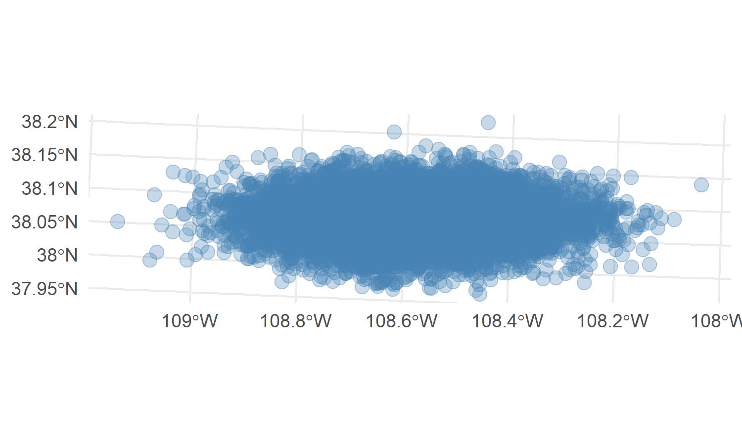
ggplot()+
  geom_sf(data = sf_obj, color = "steelblue", size = 3, alpha = 0.3)+
  theme_minimal()

The plot looks very similar to the xy plot (they should be the same), but now the points are projected. If you look at the lines behind the points you see that they are slightly askew.

Make a empty raster

Now we will create an empty raster that we will use to calculate the kernel density from. The resolution we set will be the resolution of the kernel density. We will use the raster() function from the raster package to make the raster.

empty_kernel_grid<-raster(ext = extent(sf_obj), resolution = 200, crs = st_crs(sf_obj))

Next we will take our points that we created and use the fun = 'count' parameter in the rasterize function from the to count all the points that fall within a given raster cell. We will also tell rasterize to use the empty_kernel_grid raster for the bounds of the raster.

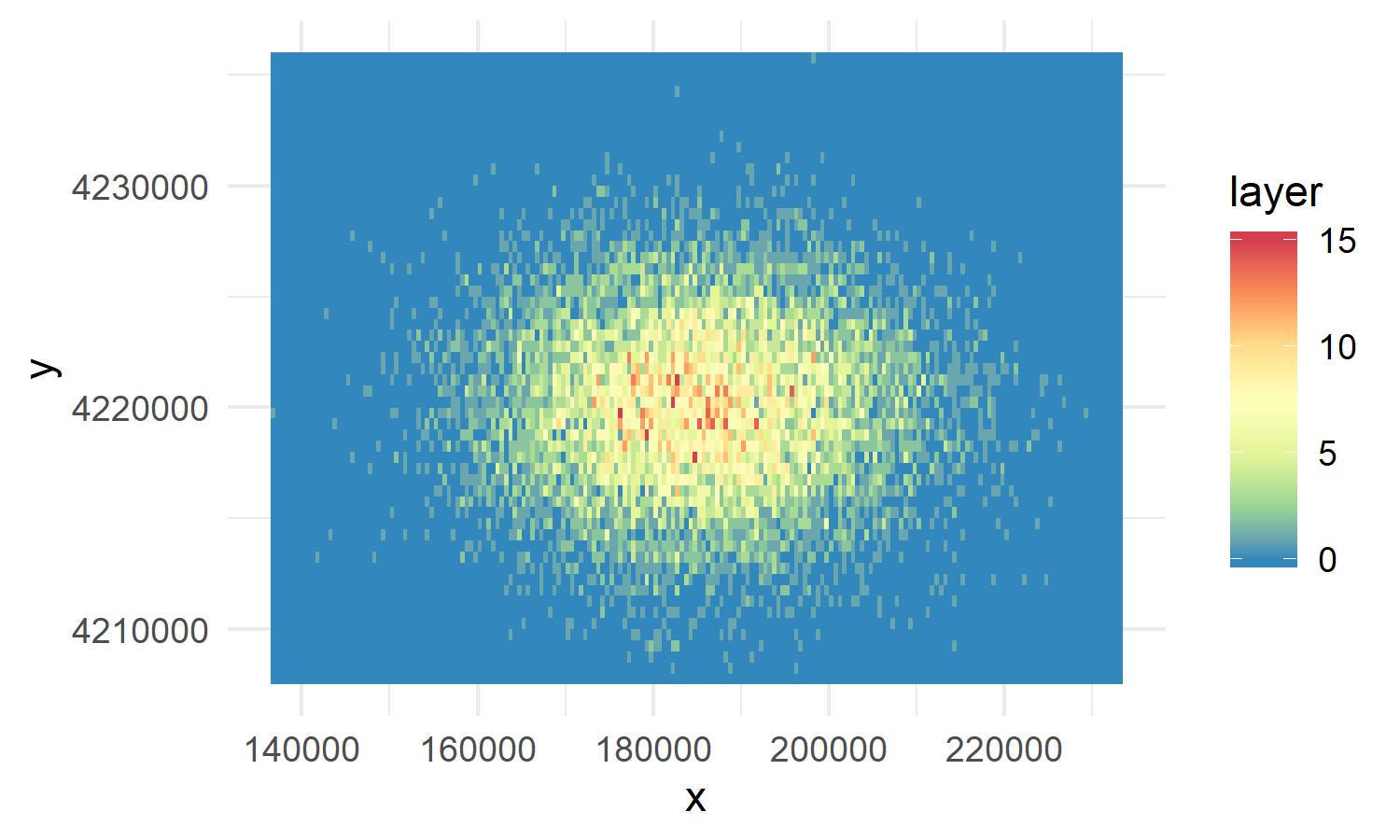
kernel_density<-rasterize(coordinates(as_Spatial(sf_obj)), empty_kernel_grid, fun='count', background = 0)

To plot a raster you with ggplot, you first must convert the raster to points with rasterToPoints.

library(RColorBrewer)
point_raster<-as_tibble(rasterToPoints(kernel_density))

ggplot(point_raster, aes(x = x, y=y))+
  geom_raster(aes(fill = layer))+
  theme_minimal()+
  scale_fill_distiller(palette = "Spectral")

Even though we had a mass to start, now we see that certain 200m areas are mor dense than other.