Extract Raster Values
Below is a method to use the raster package extract() function to get a subet of rasterBrick values. To be specific, I need to extract all raster values that are within a polygon boundary. In the past I have used crop(), mask() and then the getValues() functions from the raster package to subset data values within a polygon. But that method returns a data frame with a ton of NA values (anything outside of the crop area in the raster is an NA). This is fine most of the time but the current project that I am working on requires almost all of the memory on my computer. I'm working with extremely large rasters (2Gb). Removing the NA values after the crop(), mask(), and getValues() process crashes my computer. So I need a more effecient process.
Unlike mask(), crop() and getValues(), extract() just extracts the values inside the polygon. There is no need to remove NAs.
All processes below will rely on the raster package. So load that first.
library(raster)Extract from an extent.
Lets create a raster that we can use to extract raster values from.
r <- raster(ncol=36, nrow=18, vals=1:(18*36))
r

# class       : RasterLayer
# dimensions  : 18, 36, 648  (nrow, ncol, ncell)
# resolution  : 10, 10  (x, y)
# extent      : -180, 180, -90, 90  (xmin, xmax, ymin, ymax)
# coord. ref. : +proj=longlat +datum=WGS84 +ellps=WGS84 +towgs84=0,0,0
# data source : in memory
# names       : layer
# values      : 1, 648  (min, max)
Create clip extent that we can exract from.
ext<-extent(90,170,-60,0)Plot to see if the clip extent overlays the raster.
plot(r)
plot(ext,add=T)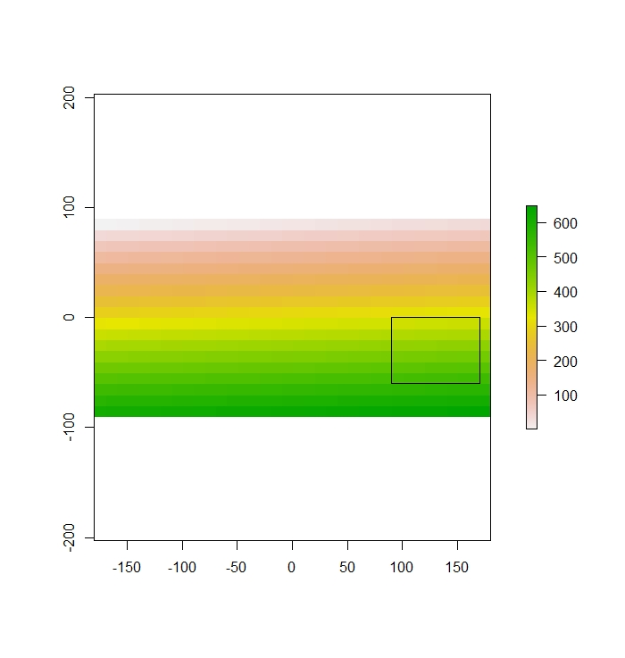
Then we use extract() to get all of the values within the extent.
extracted<-extract(r,ext)Extract returns a vector in this case.
extractedreturns
[1] 352 353 354 355 356 357 358 359 388 389 390 391 392 393 394 395 424 425 426 427 428 429 430 431 460 461 462 463 464 465 466 467 496 497 498
[36] 499 500 501 502 503 532 533 534 535 536 537 538 539
Extract from a stack.
That worked pretty well. But I rarely need to extract a raster with a single layer. I typically need to extract a raster with upwards of 10 to 20 layers. Let's try to do a stack extract.
First, add layers to the raster.
st<-stack(r, sqrt(r), r/r, r*r*r)
names(st)<-c("base", "base_sq_rt", "r_divided", "r_cubed")
Then extract the stack.
extracted_st<-extract(st, ext)
extracted_st

#      base base_sq_rt r_divided   r_cubed
#[1,]  352   18.76166         1  43614208
#[2,]  353   18.78829         1  43986977
#[3,]  354   18.81489         1  44361864
#[4,]  355   18.84144         1  44738875
#[5,]  356   18.86796         1  45118016
#[6,]  357   18.89444         1  45499293
#[7,]  358   18.92089         1  45882712
#[8,]  359   18.94730         1  46268279
#[9,]  388   19.69772         1  58411072
#[10,]  389   19.72308         1  58863869
#[11,]  390   19.74842         1  59319000
#[12,]  391   19.77372         1  59776471
#... many more rows
Extract from polygon
In reality though, I will rarely need to extract from a exten, rather, I will need to extract from a polygon or multiPolygon. First, let's try to extract based on a polygon.
First, create the polygon
x_coord<-c(70, 20, -50, -20)
y_coord<-c(50, 60, 20, -30)

xym <- cbind(x_coord, y_coord)

p <- Polygon(xym)
ps <- Polygons(list(p),1)
sps <- SpatialPolygons(list(ps))
Make sure there is overlap
plot(r)
plot(sps, add=T)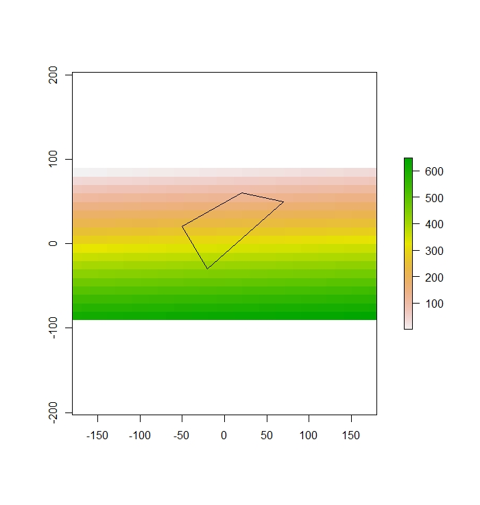
Now use the polygon to extract.
extracted_poly<-extract(st, sps)
extracted_poly
Returns:
    base base_sq_rt r_divided  r_cubed
[1,]  128   11.31371         1  2097152
[2,]  129   11.35782         1  2146689
[3,]  130   11.40175         1  2197000
[4,]  131   11.44552         1  2248091
[5,]  162   12.72792         1  4251528
[6,]  163   12.76715         1  4330747
[7,]  164   12.80625         1  4410944
[8,]  165   12.84523         1  4492125
[9,]  166   12.88410         1  4574296
[10,]  167   12.92285         1  4657463
[11,]  168   12.96148         1  4741632
[12,]  197   14.03567         1  7645373
... Many more rows
Again, it works really well.
Real world example
The prototypes above worked great. But when I tried to extract on a real world example, I ran into a problem. If your shapefile that is the extent of the extract is made up of many many polygons (a multipolygon) like mine is, it will return a list of vectors where each vector represents the values within each polygon. In my case I want all of the values to be returned in the same vector.
To do this, I first had to dissolve the polygons using the maptools() package. Then I ran extract.
Example:
# Function paramaters:
## * tile name = the name of the tile to subset training dataset from
## * folder_of_tiles = the file path to the folder that contains the tiles
## * file_path_to_shape = the file path to the shapefile.
### Notes: This function has three steps
#### 1. reads single tile, creates an NDVI layer and merges the ndvi layer into the tile
#### 2. read the shapefile and rasterizes it
#### 3. extracts the data within the shapefile training polygons.
#### 4. Write the data to a file to be read in at a later time.

subset_training_data_from_tile<- function( tile_name, folder_of_tile, file_path_to_shape){


  # read raster make ndvi layer and add it to the brick.
  raster<-brick(paste0(paste(folder_of_tiles, tile_name ,sep="/"), ".tif" ))
  ## Rename Bands for ease of calculation
  names(raster)<-c("b1", "b2", "b3", "b4")
  ## create NDVI layer
  ndvi<-overlay(raster$b4, raster$b1, fun=function(x,y){(x-y)/(x+y)})
  ## Merge NDVI and the tile imagery
  cov<-addLayer(raster,ndvi)


  # parse and read shapefile

  ## split file path based on "/"
  temp<-stringr::str_split(file_path_to_shape, "/")
  ## Put in split file path into Read OGR to read shapefile and assign to variable.
  temp2<-readOGR(dsn=paste(head(temp[[1]], -1) , collapse = "/"), layer=paste(tail(temp[[1]], 1)))
  ## convert the Class in shapefile to numeric
  temp2@data$code<-as.numeric(temp2@data$Class)
  temp2@data$dissolve<-1
  ## crop the shapefile to the extent of the current tile
  ### Then pipe to rasterize function so the the shape is converted to a raster using the field code to populate fields...with the same projection and tile size as the tile (represented by just the ndvi layer here)
  shape<-raster::crop(temp2, extent(cov))
  ## Rasterize shape to add to cov
  shape_raster<-rasterize(shape, cov, field="code")
  ## Dissolve shape for extract.
  shape_dissolve<-unionSpatialPolygons(shape, shape@data$dissolve)


  ## add shape to cov
  cov_shape<-addLayer(cov,shape_raster)

  ## Rename all columns with...
  names(cov_shape)<-c("b1", "b2", "b3", "b4", "ndvi", "class")

  # Remove unneeded objects from memory to free up compute power
  rm(ndvi, temp, temp2, raster)

  # set up dataset to be exported
  ## Crops the covariate to the shape extent.  This step may seem redundent from the step above, where we cropped the shapefile to the extent of the tile, but it is necessary to decrease the size of processed data as much as possible.
  data_to_be_modeled<-raster::extract(cov_shape, shape_dissolve)[[1]]%>%
    ## convert to dataframe
    as_tibble()

  ## Save resulting dataset to file to be read in the next function.
  saveRDS(data_to_be_modeled, paste0("training_datasets2/", tile_name, "training_data.rds"))

  ## Remove the rest of the objects to clear memory after write happens.  If you don't do this objects get built up in memory and will eventaully make the function fail.
  rm(data_to_be_modeled)
}