Colorado Avalanches By The Numbers in R

A look at avalanches in Colorado. Please not I'm not an avalanche expert, so please take these interpretations with a healthy dose of skepticism.

Avalanche Observations by Aspect

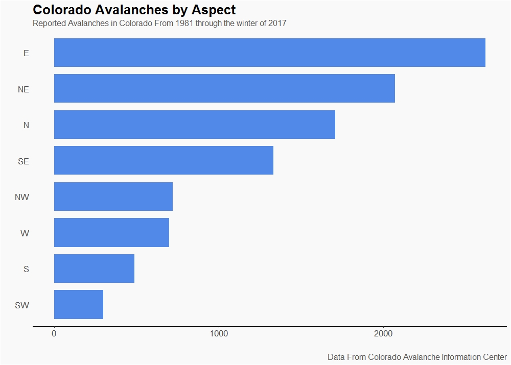
North to southeast facing are the most likely to have avalanches. This confirms what we know: snow layers that are not exposed to the sun tend to develop persistent week layers. However it is important to note that avalanches occur on all aspects.

Avalanche Observations by Elevation

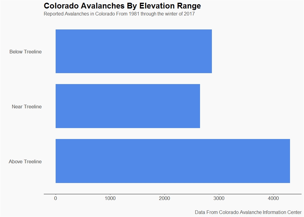
The vast majority of avalanches occur above tree line. Elevations at or below tree line have a similar number of avalanches. It would be interesting to know if there is a better way to break down avalanches by elevation. It looks to me that you could interpret this data to show that avalanches are just as likely to occur in the trees as they are above tree line. I wonder if areas well below tree line have fewer avalanches? Regardless, avalanches occur at all elevations.

Avalanche Observations by Mountain Range

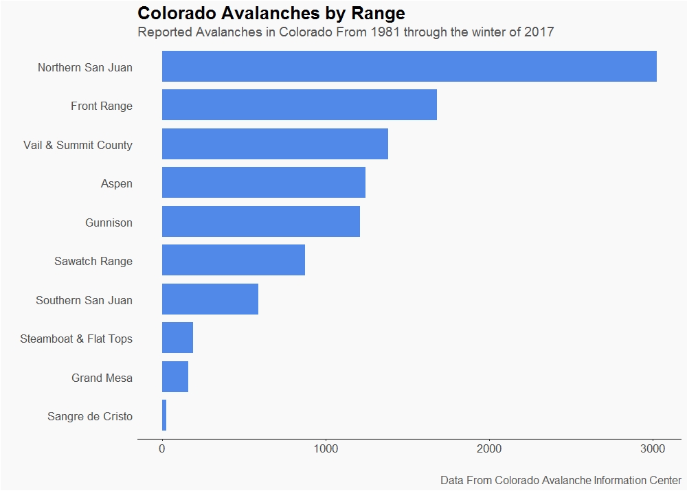
The Northern San Juans have twice as many avalanches as any other mountain range in Colorado. It would be better if we looked at this in context of area. The North San Juan is one of, if not the, biggest ranges according to how the Colorado Avalanche Information Center divides up mountain ranges in Colorado. For example Vial and Summit County also experience many Avalanches. But Vail and Summit county range is, at least based on just looking at CAICs maps, less than half the size of Northern San Juan. You would think then that Vail may be as susceptible to avalanches as the Northern San Juan. And far more people live in the Vail and Summit County areas than live in the Northern San Juans. Also, area visibility could be a factor we cannot control for. So don't read too much into this analysis.

The Takeaway

Avalanches can occur in all mountain ranges in Colorado, on all aspects, at all elevations.

Be safe out there.

The Scripts

For the most up to date scripts check out the repo: avalanche_analysis

library(tidyverse)
data<-read_csv("https://raw.githubusercontent.com/mschmidty/r_projects2/master/avalanche_caic/CAIC_avalanches_1981-11-01_2018-12-02.csv")

Aspect Graph

data%>%
  filter(Asp!="All", Asp!= "Unknown", Asp!="U")%>%
  group_by(Asp)%>%
  summarize(perc=n())%>%
  arrange(desc(perc))%>%
  ggplot(aes(x=reorder(Asp,perc), y=perc))+
    geom_bar(stat="identity", fill="#5089E8", width=0.8,position = position_dodge(width=0.2) )+
    coord_flip()+
    theme_classic()+
    xlab("")+
    ylab("")+
    labs(title="Colorado Avalanches by Aspect",
         subtitle = "Reported Avalanches in Colorado From 1981 through the winter of 2017",
         caption = "Data From Colorado Avalanche Information Center")+
    theme(axis.line.y=element_blank(),
          axis.ticks.y=element_blank(),
          text=element_text( family="Source Sans Pro", size=16),
          plot.title=element_text(face="bold"),
          plot.subtitle=element_text(size=12, color="#555555", family="Source Sans Pro Light"),
          plot.caption=element_text(size=12, color="#555555"),
          plot.background = element_rect(fill = "#f9f9f9"),
          panel.background = element_rect(fill="#f9f9f9"))

Elevation Chart

positions <- c("Above Treeline", "Near Treeline", "Below Treeline")
data%>%
  filter( Elev!="All", Elev!="U")%>%
  mutate(Elev_long = ifelse(Elev==">TL", "Above Treeline", ifelse(Elev=="<TL", "Below Treeline", "Near Treeline")))%>%
  group_by(Elev_long)%>%
  summarize(perc=n())%>%
  arrange(desc(perc))%>%
  ggplot(aes(x=Elev_long, y=perc))+
    geom_bar(stat="identity", fill="#5089E8", width=0.8,position = position_dodge(width=0.2) )+
    coord_flip()+
    scale_x_discrete(limits = positions)+
    theme_classic()+
    xlab("")+
    ylab("")+
    labs(title="Colorado Avalanches By Elevation Range",
         subtitle = "Reported Avalanches in Colorado From 1981 through the winter of 2017",
         caption = "Data From Colorado Avalanche Information Center")+
    theme(axis.line.y=element_blank(),
          axis.ticks.y=element_blank(),
          text=element_text( family="Source Sans Pro", size=16),
          plot.title=element_text(face="bold"),
          plot.subtitle=element_text(size=12, color="#555555", family="Source Sans Pro Light"),
          plot.caption=element_text(size=12, color="#555555"),
          plot.background = element_rect(fill = "#f9f9f9"),
          panel.background = element_rect(fill="#f9f9f9"))

Range Chart

data%>%
  rename(Zone=6)%>%
  filter(Zone!=is.na(Zone))%>%
  group_by(Zone)%>%
  summarize(perc=n())%>%
  arrange(desc(perc))%>%
  ggplot(aes(x=reorder(Zone, perc), y=perc))+
    geom_bar(stat="identity", fill="#5089E8", width=0.8,position = position_dodge(width=0.2) )+
    coord_flip()+
    theme_classic()+
    xlab("")+
    ylab("")+
    labs(title="Colorado Avalanches by Range",
         subtitle = "Reported Avalanches in Colorado From 1981 through the winter of 2017",
         caption = "Data From Colorado Avalanche Information Center")+
    theme(axis.line.y=element_blank(),
          axis.ticks.y=element_blank(),
          text=element_text( family="Source Sans Pro", size=16),
          plot.title=element_text(face="bold"),
          plot.subtitle=element_text(size=14, color="#555555", family="Source Sans Pro Light"),
          plot.caption=element_text(size=12, color="#555555"),
          plot.background = element_rect(fill = "#f9f9f9"),
          panel.background = element_rect(fill="#f9f9f9"))